
Sarah O’Connor’s We Are Not Machines: The Fight for the Future of Work accompanied me on my summer holiday, but it has continued to unsettle how I think about work. It is an engaging, accessible book, and precisely the kind that prompts a recalibration of what you want your own work to be about. In the age of AI, it offers a useful lens for deciding what we should automate, what we should protect, and who gets to make those choices.
I am not anti-AI; I am pro-human. I routinely use AI tools, my research involves designing hardware for AI, and I welcome their use where they genuinely enhance life. The difficult questions are which parts of life they enhance, who gets to decide, and what exactly we mean by “enhancement”.
O’Connor examines the intersection of work and technology through our collective struggle to preserve some of our most cherished human traits: “to pass skill and knowledge from one generation to the next; to create, and to delight one another with our creations; to care for each other when we are too weak to care for ourselves”. The book is structured into three sections: “Mind”, “Body”, and “Soul”, which explore autonomy in cognitive work, safety in physical labour, and the intrinsic value of skill, creation, and care. Moving across warehouses, mines, care homes, and creative studios, O’Connor repeatedly returns to three questions: who shapes technology and its adoption, under what incentives, and in whose interests?
For me, the book’s deeper lesson is that these choices are rarely individual. What workers can protect depends on whether they have any collective power over how technology is introduced. The title itself comes from the 1969-70 strike by miners at the Swedish state-owned company LKAB. Their rallying cry was Vi är ej maskiner: we are not machines. Tellingly, the book’s most hopeful narratives are those in which people act collectively to reclaim agency over how their work is organised.
Craft and “Vibe Knitters”
A concept that particularly resonated with me is O’Connor’s use of Karri Saarinen’s account of craft: “the deliberate attention put into making something excellent, not because someone is checking, but because it matters to the maker”. O’Connor also cites Saarinen’s wider economic point that when something becomes cheaper to build, the default outcome is often simply to build more of it, making us less critical of what actually deserves to exist. I recognise this tension from my own vibe coding. The speed and ease are exhilarating, yet they risk detaching the act of production from the rigorous exercise of judgement.
O’Connor restores the historical context around the stockingers who became Luddites. Far from being ignorant reactionaries smashing unfamiliar machines, they were highly skilled framework knitters reacting against particular uses of machinery that degraded both their trade and its products. She refers to the employment of unapprenticed “colts” to turn out cheap goods as “vibe knitters” of their day. The historical question, then as now, is about the social relations in which machines are deployed, the kinds of work they enable, and the products they are used to create.
This discussion connects to a much older debate about the division of labour. O’Connor cites Frederick Winslow Taylor, whose The Principles of Scientific Management sought to convert workers’ accumulated craft knowledge into “rules, laws, and formulae” held and applied by management, displacing individual judgement. Against this, she places John Ruskin’s 1853 warning in “The Nature of Gothic”: it is not merely labour that is divided, but people themselves, broken into “fragments and crumbs of life”.
Karl Marx’s theory of alienation has much to add to this discussion. In the 1844 manuscripts, Marx describes four connected dimensions of alienation: the worker is estranged from the product, from the activity of labour, from other people, and from the human capacity for free, conscious creation. His observation that the worker’s activity “belongs to another” and is “a loss of his self” is therefore not simply a claim about who owns the product. It highlights the worker’s estrangement from their own activity – work experienced as external, compelled, and no longer self-directed. By 1848, Marx and Friedrich Engels wrote in The Communist Manifesto that the worker “becomes an appendage of the machine”.
Each of these thinkers helps illuminate what changes when workers are separated from meaningful responsibility for both their labour and its result. Specialisation enables production on a scale impossible for a solo craftsperson. But those gains ring hollow when work is so fractured that nobody can see, or care about, the whole. Something human is extracted from the process, even as measurable output soars. Unless, perhaps, there is collective and living control over the entire enterprise.
What Should We Automate?
O’Connor quotes an interviewee who poses a striking question: why are we so eager to automate the cognitive activities our minds excel at, and which nourish our minds, rather than the physical tasks our bodies struggle with and which cause physical damage? This question stayed with me throughout the holiday.
Expanding on this, she cites Andreas Schleicher on generative AI in education. A system can effortlessly throw an answer back at us without revealing its provenance or how it was constructed. I recently experienced my own somewhat jarring version of this. I found myself spending more time investigating the intellectual lineage of a mathematical proof generated by GPT-5.5 than I spent proving the theorem from scratch in Lean. It inverted my sense of what takes time in research. Producing the formal mathematical object was almost instantaneous; establishing its origins, understanding its mechanics, and deciding whether I actually thought it illuminating remained stubbornly slow.
This is not necessarily a negative development, but it shifts where the craft lies. Unless we notice that shift, we risk mistaking possession of an answer for understanding.
Seeing the Whole Person
Perhaps the book’s most compelling case study is the Dutch home-care organisation Buurtzorg. Its model relies on small, self-managing teams of nurses who take holistic responsibility for the entire care process. A highly trained nurse might administer complex medication, dress a wound, and then make the patient a sandwich. Viewed through a strictly Taylorist lens, making a sandwich is a gross misallocation of expensive skill and ought to be delegated to cheaper labour. Viewed as part of human care, however, it becomes an opportunity to observe how that person is living and assess their broader needs. The simple task is inseparable from the skilled one.
The same pattern extends beyond nursing. I see it in the creeping deskilling of teaching in England, where the educator’s role is increasingly carved into separately managed tasks. An Ofsted study of teacher wellbeing found that limited influence over policy – teachers feeling “done to” rather than “worked with” – contributed to a sense of de-professionalisation. The same logic shapes the ticketing systems through which large institutions, including my own, manage HR and ICT support. It also shapes higher education, where interactions with staff and students are increasingly packaged, routed, and siloed. In each case, relationships that depend on continuity and judgement are divided into discrete, measurable transactions.
Specialists matter, and a functioning ticketing system is preferable to chaos. Yet any honest accounting of efficiency must include the hidden cost of nobody seeing the person – or the problem – as a whole. It must also account for what workers lose when their roles become too narrow for them to exercise judgement or care about the outcome – and, centrally, when they cannot reach beyond those roles through collective control of the production process as a whole.
Who Is the “We”?
O’Connor skewers what she describes as a cliché that technologies are “only tools” and that what matters is how we choose to use them. Her counter-question is simple: who exactly belongs to the “we” making those choices?
It is striking that almost all the battles for human-centred work detailed in the book are collective ones, even when their victories are ultimately codified as individual rights. The Swedish miners did not optimise their relationship with machinery through individual negotiation. More recently, during its 148-day strike, the Writers Guild of America won rules in the 2023 agreement governing AI: AI could not write or rewrite literary material under the agreement; AI-generated material was not source material; and writers could not be required to use AI. These were foundational choices about technology, won through organised labour.
Because such victories are codified as rights exercised by individuals, their collective origins are easy to forget. Nicos Poulantzas is useful here. In State, Power, Socialism, he treats the state as a material condensation of the balance of forces among classes and class fractions. This offers one way of seeing how rights that appear to belong to isolated individuals can bear the imprint of collective struggle. The right may be granted and exercised individually; the power that made it possible was collective.
The “we” defining technological choice must include those actually performing the work. For people divorced from the ownership and control of the technology, exhortations to preserve their craft are nearly useless if they control neither the tools nor the targets and metrics by which their work is judged.
More Than Machines
The final chapters include perhaps the book’s most unsettling idea: that what some call artificial general intelligence (AGI) might arrive not because machines advance, but because humans retreat from what we are capable of when faced with apparently superior machine performance. Organisations may treat us as machines, but we may also come to understand ourselves as defective machines, slow and inconsistent approximations of systems whose strengths we have adopted as the gold standard.
I closed the book wanting to identify – and ruthlessly prioritise – the crafts I most enjoy, at work and beyond. I remain eager to use AI to automate genuine human drudgery. Yet the current temptation is to automate whatever is easiest to automate, rather than what we actually wish to relinquish, on the vague promise that doing so will free us up for… what exactly?
Much of life’s joy resides in craft. Those of us fortunate enough to retain some autonomy over our work and lives should think carefully before surrendering it. O’Connor’s narratives show that preserving human craft requires both individual choice and collective action. Remaining more than machines is not merely a personal preference, it is a collective and deeply political task.
Sources and further reading
Quotations not otherwise linked are drawn from Sarah O’Connor’s We Are Not Machines: The Fight for the Future of Work.
People
- Sarah O’Connor – Financial Times profile
- Karri Saarinen – Linear profile
- Frederick Winslow Taylor – biography
- John Ruskin – biography
- Karl Marx – Stanford Encyclopedia of Philosophy
- Friedrich Engels – biography
- Andreas Schleicher – biography
- Nicos Poulantzas – biography
Primary texts
- Sarah O’Connor, We Are Not Machines: The Fight for the Future of Work
- Frederick Winslow Taylor, The Principles of Scientific Management
- John Ruskin, “The Nature of Gothic”, in The Stones of Venice, Volume II
- Karl Marx, “Estranged Labour”, in the Economic and Philosophic Manuscripts of 1844
- Karl Marx and Friedrich Engels, The Communist Manifesto, Chapter I
- Nicos Poulantzas, State, Power, Socialism
- Writers Guild of America, summary of the 2023 Minimum Basic Agreement
Broader context
- Stanford Encyclopedia of Philosophy, “Karl Marx”: alienation and human flourishing
- The Guardian review, including the origin of the book’s title
- Encyclopaedia Britannica, “Luddite”
- The 2023 Writers Guild of America strike
- Buurtzorg’s model of care
- Ofsted, Teacher well-being at work in schools and further education providers
- Lean theorem prover
AI tools were used to support copy-editing and to help collect and organise the links above.
 . For example,
  , then the unscaled vectors we can represent are the product set


 , how close is the nearest direction obtainable from the alphabet
  is better.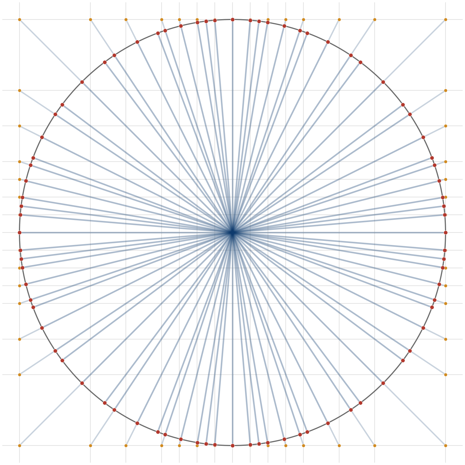
 elements. The definition
  . The quantity
  points.
  raw vectors, those vectors are not arbitrary. They arise from independent coordinate choices from the same scalar alphabet. Meanwhile, a spherical code with

 is the smaller of the number of positive and negative nonzero values in
 grows like
  , this bound tends towards
  for any fixed alphabet. In plain language: in sufficiently high dimension, every fixed scalar alphabet has some direction that it represents very badly.
 in high dimension (see above), it is more informative when comparing product codes to look at a normalised quantity such as:
 -bit alphabets. The quantity normBestAlpha n (2 ^ b) is the best normalised performance obtainable by an arbitrary
  -element scalar alphabet. The quantity normBestFpCos n b is the corresponding floating-point quantity, optimised over valid splits of exponent and mantissa bits. The constants arbConst b and fpConst b are the two asymptotic constants being compared.
 , arbitrary scalar alphabets can do strictly better than the floating-point family in this asymptotic directional metric.
 (as used in NVIDIA NVFP4), the optimised positive levels found in the paper are approximately
 , and each block is approximated as
  , where
  is a low-precision mantissa vector and
  is a scalar block scale.
 .
. , so that the represented block becomes
  .
. . Then
  .
. , so that
  is the fraction of the ideal projected vector’s energy contained in block
  (the proof is included at the end of this post).
 are across blocks. If all blocks were rescaled by the same factor, direction would be unchanged.
![x_b \in [2^{-1/2},\,2^{1/2}]](https://s0.wp.com/latex.php?latex=x_b+%5Cin+%5B2%5E%7B-1%2F2%7D%2C%5C%2C2%5E%7B1%2F2%7D%5D&bg=ffffff&fg=000000&s=0&c=20201002) .
. can be, when all the
 ![[2^{-1/2},\,2^{1/2}]](https://s0.wp.com/latex.php?latex=%5B2%5E%7B-1%2F2%7D%2C%5C%2C2%5E%7B1%2F2%7D%5D&bg=ffffff&fg=000000&s=0&c=20201002) .
.![[\ell,u]](https://s0.wp.com/latex.php?latex=%5B%5Cell%2Cu%5D&bg=ffffff&fg=000000&s=0&c=20201002) , then
, then (proof at the end of this blog post).
 ,
,  , so
, so  , and therefore
 .
. .
. of the ideally scaled one.
 .
. , and
, and  .
. .
. , so that
  , the numerator becomes
  and the denominator becomes
  , giving
 .
. 
![x_b \in [\ell,u]](https://s0.wp.com/latex.php?latex=x_b+%5Cin+%5B%5Cell%2Cu%5D&bg=ffffff&fg=000000&s=0&c=20201002) with
with  .
. .
. . Since each
 ![x_b\in[\ell,u]](https://s0.wp.com/latex.php?latex=x_b%5Cin%5B%5Cell%2Cu%5D&bg=ffffff&fg=000000&s=0&c=20201002) , we have
, we have .
. .
. .
. .
. also lies in the interval
  over
over ![\mu\in[\ell,u]](https://s0.wp.com/latex.php?latex=%5Cmu%5Cin%5B%5Cell%2Cu%5D&bg=ffffff&fg=000000&s=0&c=20201002) .
. , the harmonic mean of
  and
and  ,
, .
. .
. ,
, .
. whose coordinates are partitioned into blocks
  .
. is invariant to rescaling of
  of a vector into its magnitude and direction, but applied locally within blocks.
 , then scaling it appropriately produces a good approximation of that block.
 . Then
  is the orthogonal projection of
  .
. .
. , which we can think of as the fraction of the vector’s energy contained in block
  .
. represent how much of the vector’s energy lies in each block. Blocks that contain very little energy contribute very little to the final direction. The important consequence is that direction errors do not accumulate catastrophically across blocks. Instead, the overall directional error simply depends on a weighted average of the block direction errors. In other words, if block number formats preserve the directions of individual blocks, they automatically preserve the direction of the entire vector.
 where
where  is orthogonal to
  .
. .
. .
. , we obtain
 .
. .
. .
. , and writing
 .
. , we obtain
 .
.

 . It is the set of objects we are trying to learn about.
 over
over  is a set of concepts, i.e.
  , where
  denotes power set. We will follow Kearns and Vazirani and also use
  .
. is not. However, it doesn’t seem a jump to allow for unknown target class, in an appropriate approximation setting – I would welcome comments on established frameworks for this.
 is a probability distribution over
  taking a concept class and a distribution, and returning a labelled example
  where
where  is drawn randomly and independently from
  with reference to a target concept class
  , where
  denotes probability.
 where
where  is a finite alphabet of symbols (or – following the
  with each string from a representation alphabet
  . We similarly associate a size with each concept
  .
. be representation classes classes over
  . We say that concept class
  and
and  , with probability at least
  , outputs a hypothesis
  with
with  .
. and
and  be representation classes classes over
  , where
  for all
  or
or  . Let
. Let  ,
,  , and
, and  . We say that concept class
  over any distribution
  ,
,  , and
, and  , and
, and (the ‘probably’ bit) and
  (the ‘approximate’ bit). The first of these captures the idea that we may get really unlucky with our calls to the oracle, and get misleading training data. The second captures the idea that we are not aiming for certainty in our final classification accuracy, some pre-defined tolerance is allowable. Thirdly, note the requirements of efficiency: polynomial scaling in dimension, in size of the concept (complex concepts can be harder to learn), in error rate (the more sloppy, the easier), and in probability of algorithm failure to find a suitable hypothesis (you need to pay for more certainty). Finally, and most intricately, notice the separation of concept class from hypothesis class. We require the hypothesis class to be at least as general, so the concept we’re trying to learn is actually one of the returnable hypotheses, but it can be strictly more general. This is to avoid the case where the restricted hypothesis classes are harder to learn; Kearns and Vazirani, following
  and
and  be real constants. An algorithm is an
  -Occam algorithm for
  of cardinality
  is consistent with
 ). Note, however, that there is nothing in this definition that suggests predictive power on unseen samples.
 . Then there is a constant
  such that if
  , then
  and, with probability at least
  , the output
  .
. . Of course, one needs sufficient observations (the complex lower bound on
  that are realised by
  .
. then forms a kind of fingerprint of
  .
. is the maximum cardinality that’s possible, i.e. the set of behaviours is all possible behaviours. So we can think of a set as being shattered by a concept class iff there’s no combination of inclusion/exclusion in the concepts that isn’t represented at least once in the set.
 , is the cardinality of the largest set shattered by
  .
. . Let
. Let  such that
  .
. examples in the worst case.
 and in which the edges are always from some layer
  . Vertices at layer 0 have indegree 0 and are referred to as input nodes. Vertices at other layers are referred to as internal nodes. There is a single output node of outdegree 0.
  -composition). For a layered DAG
  with each vertex
  in
in  internal nodes, each of indegree
  . Let
. Let  of VC dimension
  be the
  .
. and
and  such that
  satisfies
  .
. we define
  to be the distribution obtained by flipping a fair coin and, on a heads, drawing from
  . Similarly, we define
  to be the distribution obtained by drawing examples from
  . Similarly,
  contains new information about
  . Let the distributions
  be defined above, and let
  ,
,  ,
,  . Then if
  , it follows that
  .
. is monotone and strictly decreasing over
  . Hence by combining three hypotheses with only marginally better accuracy than flipping a coin, the boosting lemma tells us that we can obtain a strictly stronger hypothesis. The algorithm for (strong) PAC learnability therefore involves recursively calling this boosting procedure, leading to the majority tree – based hypothesis class. Of course, one needs to show that the depth of the recursion is not too large and that we can sample from the filtered distributions with not too many calls to the overall oracle
  extends the earlier idea of an oracle with an additional noise parameter
  . This oracle behaves in the identical way to
  except that it returns the wrong classification with probability
  .
. ,
,  and
and  with
with  , given access to a noisy oracle
  then
then  takes queries of the form
  where
where  and
and  , and returns a value
  satisfying
  where
where ![P_\chi = Pr_{x \in {\mathcal D}}[ \chi(x, c(x)) = 1 ]](https://s0.wp.com/latex.php?latex=P_%5Cchi+%3D+Pr_%7Bx+%5Cin+%7B%5Cmathcal+D%7D%7D%5B+%5Cchi%28x%2C+c%28x%29%29+%3D+1+%5D&bg=ffffff&fg=000000&s=0&c=20201002) .
. ,
,  and
and  such that: for any
  , the following hold. (i) For every query
  made by
  can be evaluated in time
  , and
, and  , (ii)
  , (iii)
  . The oracle must return an estimate of the probability that this predicate holds (where the probability is over the distribution over
  , then by Occam’s Razor (above) polynomially evaluable hypothesis classes are also polynomially-learnable ones. So we will need to do two things: focus our attention on polynomially evaluable hypothesis classes (or we can’t hope to learn them polynomially), and make a suitable hardness assumption. The latter requires a very brief detour into some results commonly associated with cryptography.
 . We define the cubing function
  by
by  . Let
. Let  define
  is bijective, so we can talk of a unique discrete cube root.
  and
and  not a multiple of 3, where
  . Given
  and
and  as input, output
  , there is no algorithm that runs in time
  that solves the discrete cube root problem with probability at least
  , where the probability is taken over randomisation of
  such that each
  has
has  Boolean inputs and at most
  nodes, the depth of
  is not efficiently PAC learnable (using any polynomially evaluable hypothesis class), and even if the weights are restricted to be binary.
 , i.e. not just to be shown randomly selected examples but take charge and test their understanding of the concept.
 , returning this counterexample if so.
 .
.
