Probably Approximately Correct

This Christmas, one of the books I read during my holiday was Leslie Valiant’s book Probably Approximately Correct, if not quite a truly general readership-oriented book, then certainly one suitable for anyone with a scientific background and equally suitable for adults and teens.

Valiant needs no introduction to those with a background in computer science – for those outside the field, you can read about his deep contributions on his Wikipedia page. Inspired by the work of Turing, in this book (from 2013) he presents some wide-ranging thoughts on the Probably Approximately Correct (PAC) framework for understanding learning kicked off by his paper from 1984, presenting the concept as fundamental to learning as it occurs naturally. He deals with both “learning of the species, through evolution” and the more commonly considered “learning of the individual” within the same algorithmic framework – which he calls “ecorithms” – identifying the weaker learning behaviours possible in the former setting.

This is a great book, full of ideas and interesting philosophical discussion points. The key exciting elements to me relate to the use of computational complexity arguments to shed light on the different classes of function that can be learnt in a resource-constrained setting, as per the original PAC technical work, and the broader philosophical conclusions Valiant draws from this. Some particular ideas that stood out to me as worthy of further thought (my own list, Valiant does not prioritise these ideas):

The modularity of biological systems as a side-effect of the limited learnability (through evolution) of large-scale non-modular systems
The idea that “artificial” in “artificial intelligence” should not be considered as defining “the material basis of the realisation” (i.e. an intelligence may be natural or artificial in a computer, for example), but rather in the way knowledge is obtained from the environment. The key distinction for Valiant is whether we are trying to reproduce learning the same way this happens in nature (this not “artificial” for Valiant) or whether we are trying to do something different, e.g. shortcutting evolutionary processes (imagine a classical Chess-playing AI).
The idea that unsupervised learning is not a natural phenomenon, because the training is present even in the natural state, e.g. via evolutionary fitness for evolution-as-learning.
Some interesting thoughts on the role of ecorithms in the development of human culture and knowledge, and how humans have tipped the balance from evolutionary learning to stronger forms of algorithmic learning through their ability to pass on culture and knowledge to future generations.

In addition to Valiant’s ideas, a few thoughts that struck me while reading the book, which I wonder whether others have considered in more depth:

During our work together on resource-constrained model-predictive control, my friend and colleague Eric Kerrigan would often say to me that the best resource-constrained model for an open-loop system may be very different to the best resource-constrained model for that same system in a closed-loop setting for control purposes. It strikes me that the notion of fitness used by Valiant to pose evolvability as a learning might be further enriched by thinking along these lines, especially as the species being evolved changes the environment within which it lives.
Valiant argues that questions such as “can a computer have free will?” and “is a termite conscious?” are meaningless “because the concepts the words describe have meanings only for the distribution of examples from which they have been PAC learned”. This seems a step too far for me, not least because many of the most creative leaps I’ve seen in thought have come from applying ideas in one area to a completely distinct one. It would be useful, I think, to make the assertion more precise and to explore it a bit more deeply.
Throughout the book, Valiant makes heavy use of the classical “polynomial versus non polynomial” approach to characterising complexity (e.g. arguing that useful learning takes polynomial time to learn classification of exponential items). This is, as one would expect, well justified in terms of the robustness of these classes, but it leaves me wondering what we lose by taking an asymptotic approach to drawing conclusions in the non-asymptotic settings of animals and their behaviours.

I would recommend this book to all. When I visit sixth forms to talk about my work and about engineering at Imperial, I’m often asked by teachers and students if I have recommendations for accessible but deep reading. I will be recommending Valiant’s book in the future.

Notes on Model Theory

This summer, I decided to read something about Model Theory. Aware of my limited time, I decided to aim for a slim volume as a guide, so went for An Invitation to Model Theory by Jonathan Kirby.

Here I collect some notes I made while reading Kirby, completely biased to my own interests. Definitions and theorems largely follow the book, but have often been tweaked by me to make my notes more self-contained. I’ve also tried to ‘sloganise’ each of the originally-unnamed theorems in a way that helps me grasp their essence. Additional commentary around the definitions and theorems is mine, and I’ve added a couple of extra definitions to make things easier for me to read back in the future. Of course there is some risk that I’ve introduced errors or lack of clarity, in which case I’m sure the fault lies with me not with the book – please do reach out if you spot anything.

What this post will discuss

We will look at defining basic syntactical objects, terms and formulas, and their interpretations (all in first-order logic). We will look at ideas relating to whether mathematical structures can be distinguished via the truth of formal sentences, including embedding of one structure inside another. We will look at results guaranteeing the existence of structures (especially infinite structures) satisfying sets of such sentences. Turning this around, we’ll also look at some results on which structures can be axiomatised by such sets of sentences. We will consider the extent to which one can define a subset using first-order sentences and the relationship to quantifier elimination (see also my post including algorithms for quantifier elimination). Finally, we will look at the idea of ‘how uniquely’ mathematical structures can be described in this way.

What this post will not discuss

I have purposely not given proofs or examples. Kirby’s book of course has (most) proofs and is rich in examples, through which much of the material is developed. This means I have not discussed some really interesting results on, say, algebraically closed fields, on which Kirby spends considerable time. Those interested in how to apply some of these ideas would do well to consult the book. In addition, I have avoided the topic of types in this simple set of notes, which Kirby highlights as a “central concept in model theory”, despite the interesting results they enable later in the book, e.g. saturated models. The exception is that I included a simplified version of the Ryll-Nardzewski theorem at the end of this post (the proof given uses types) because this particular part of the theorem may be of use to me in the future and can be stated without recourse to types.

I hope to do a later blog post with some of the material using types in due course.

Languages and Structures

Definition (Language). A language $L$ consists of a set of relation symbols, a set of function symbols, a set of constant symbols and, for each relation and function symbol, a positive number known as its arity. The set of all these symbols is denoted $\text{Symb}(L)$ .

Definition ( $L$ –structure). An $L$ -structure $\mathcal{A}$ consists of a set $A$ called its domain, together with interpretations of the symbols in $L$ : for each relation symbol $R$ of arity $n$ , a subset $R^\mathcal{A}$ of $A^n$ ; for each function symbol $f$ of arity $n$ , a function $f^\mathcal{A} : A^n \to A$ ; for each constant symbol $c$ , a value $c^\mathcal{A} \in A$ .

Definition (Embedding). Let $\mathcal{A}$ and $\mathcal{B}$ be $L$ -structures. An embedding of $\mathcal{A}$ into $\mathcal{B}$ is an injection $\pi: A \to B$ s.t.: for all relation symbols $R$ of $L$ and all $a_1,\ldots,a_n \in A$ , $(a_1,\ldots,a_n) \in R^\mathcal{A}$ iff $\pi(a_1),\ldots,\pi(a_n) \in R^\mathcal{B}$ ; for all function symbols $f$ of $L$ and all $a_1,\ldots,a_n \in A$ , $\pi(f^\mathcal{A}(a_1,\ldots,a_n)) = f^\mathcal{B}(\pi(a_1),\ldots,\pi(a_n))$ ; for all constant symbols $c$ of $L$ , $\pi(c^\mathcal{A}) = c^\mathcal{B}$ .

Definition (Isomorphism). An embedding $\pi: \mathcal{A} \to \mathcal{B}$ is an isomorphism iff there is an embedding $\sigma: \mathcal{B} \to \mathcal{A}$ s.t. $\pi \circ \sigma$ is the identity on $\mathcal{B}$ and $\sigma \circ \pi$ is the identity on $\mathcal{A}$ .

Definition (Automorphism). An automorphism is an isomorphism from a structure to itself.

Terms, Formulas and their Models

Definition ( $L$ –term). The set of terms of the language $L$ is defined recursively as follows: every variable is a term; every constant symbol of $L$ is a term; if $f$ is a function symbol of $L$ of arity $n$ and $t_1, \ldots, t_n$ are terms of $L$ , then $f(t_1, \ldots, t_n)$ is a term; only something built from the preceding clauses in finitely many steps is a term.

Definition ( $L$ –formula). The set of formulas of $L$ is defined recursively as follows: if $t_1$ and $t_2$ are terms, then $(t_1 = t_2)$ is a formula; if $t_1, \ldots t_n$ are terms and $R$ is a relation symbol of $L$ of arity $n$ , then $R(t_1, \ldots t_n)$ is a formula; if $\varphi$ and $\psi$ are formulas, then $\neg \varphi$ and $\varphi \wedge \psi$ are formulas; if $\varphi$ is a formula and $x$ is a variable, then $\exists x[\varphi]$ is a formula; only something built from the preceding four clauses in finitely many steps is a formula. We will write $\varphi(x)$ for a formula with free variables $x = (x_1, \ldots x_n)$ in some defined order.

Definition ( $L$ –sentence). An $L$ -sentence is a $L$ -formula with no free variables.

Definition (Atomic formula). Formulas of the form $t_1 = t_2$ for some $L$ -terms $t_1, t_2$ or of the form $R(t_1,\ldots,t_n)$ for some relation symbol $R$ and terms $t_1,\ldots,t_n$ are atomic formulas.

Definition (Interpretation of terms). Let $\mathcal{A}$ be an $L$ -structure, $t$ be a term of $L$ , and $x = (x_1, \ldots, x_r)$ be a list of variables including all those appearing in $t$ . The interpretation of $t$ , written $t^\mathcal{A}$ is a function from $A^r$ to $A$ defined by: if $t$ is a constant symbol $c$ then $t^\mathcal{A} : x \mapsto c^\mathcal{A}$ ; if $t$ is $x_i$ then $t^\mathcal{A} : x \mapsto x_i$ ; if $t$ is $f(t_1, \ldots, t_n)$ then $t^\mathcal{A} : x \mapsto f^\mathcal{A}(t_1^\mathcal{A}(x), \ldots, t_n^\mathcal{A}(x))$ .

Definition (Interpretation of formulas). We define $\mathcal{A} \vDash \phi(a)$ (read $\vDash$ as ‘models’) recursively as: $\mathcal{A} \vDash t_1(a) = t_2(a)$ iff $t_1^\mathcal{A}(a) = t_2^\mathcal{A}(a)$ ; $\mathcal{A} \vDash R(t_1(a), \ldots, t_n(a))$ iff $(t_1^\mathcal{A}(a), \ldots, t_n^\mathcal{A}(a)) \in R^\mathcal{A}$ ; $\mathcal{A} \vDash \neg \varphi(a)$ iff $\mathcal{A} \nvDash \varphi(a)$ ; $\mathcal{A} \vDash \varphi(a) \wedge \psi(a)$ iff $\mathcal{A} \vDash \varphi(a)$ and $\mathcal{A} \vDash \psi(a)$ ; $\mathcal{A} \vDash \exists x[\varphi(x,a)]$ iff there is some $b \in A$ s.t. $\mathcal{A} \vDash \varphi(b,a)$ .

Definition ( $L$ –sentence). An $L$ -sentence is a $L$ -formula with no free variables.

Definition (Models of sentences). For a sentence $\varphi$ , if $\mathcal{A} \vDash \phi$ we say $\mathcal{A}$ is a model of $\varphi$ . For a set of sentences $\Sigma$ , we say that $\mathcal{A}$ is a model of $\Sigma$ ( $\mathcal{A} \vDash \Sigma$ ) iff it is a model of all sentences in $\Sigma$ .

Definition (Entailment). Let $\Sigma$ be a set of $L$ -sentences and $\varphi$ be an $L$ -sentence. $\Sigma$ entails $\varphi$ , written $\Sigma \vdash \varphi$ if every model of $\Sigma$ is also a model of $\varphi$ .

Note that I am using the notation for entailment used by Kirby’s book, for consistency, but computer scientist readers of my blog will want to note that this symbol is commonly also used for (the more restricted, assuming sound) ‘proves’ relation for a formal deductive system.

Definition (Deductively closed). A set $\Sigma$ of $L$ -sentences is deductively closed iff, for every $L$ -sentence $\sigma$ , if $\Sigma \vdash \sigma$ then $\sigma \in \Sigma$ .

(Again note no formal deduction in play here.)

Definition (Satisfiable). A set of sentences $\Sigma$ is satisfiable iff there exists some $L$ -structure $\mathcal{A}$ such that $\mathcal{A} \vDash \Sigma$ .

Definition (Complete). A set $\Sigma$ of $L$ -sentences is complete if, for every $L$ -sentence $\varphi$ , either $\Sigma \vdash \varphi$ or $\Sigma \vdash \neg \varphi$ .

Definition (Theory). A theory is a satisfiable and deductively closed set of $L$ -sentences.

Definition (Theory of a structure). The theory of an $L$ -structure $\mathcal{A}$ , denoted $\text{Th}(\mathcal{A})$ is the set of all $L$ -sentences which are true in $\mathcal{A}$ .

Elementary Equivalence

It’s clearly interesting to know whether structures can be distinguished by sentences:

Definition (Elementary equivalence). Two $L$ -structures $\mathcal{A}$ and $\mathcal{B}$ are elementarily equivalent, denoted $A \equiv B$ iff for every $L$ -sentence $\varphi$ , $\mathcal{A} \vDash \varphi$ iff $\mathcal{B} \vDash \varphi$ .

Compactness

Theorem (Compactness). Let $\Sigma$ be a set of $L$ -sentences. If every finite subset of $\Sigma$ has a model then $\Sigma$ has a model.

A huge amount of excitement flows from the compactness theorem, including many of the results that follow.

Proposition (Elementarily-equivalent non-isomorphic structures). Let $\mathcal{A}$ be any infinite $L$ -structure. Then there is another $L$ -structure which is elementarily equivalent to $\mathcal{A}$ but not isomorphic to it.

And so, via this route, we get wonderful non-standard models. As we will see in a moment, via the Löwenheim-Skolem theorems, there are actually many such structures.

Axiomatisable Classes

Definition (Axiomatisable class). If $\Sigma$ is a set of $L$ -sentences then denote by $\text{Mod}(\Sigma)$ the class of all $L$ -structures which are models of $\Sigma$ . The class $\text{Mod}(\Sigma)$ is axiomatised by $\Sigma$ and is and axiomatisable class. The class is finitely axiomatised if it is axiomatised by a finite set of sentences.

By compactness, we can’t capture arbitrarily sized, but finite, models (e.g. the class of all finite groups):

Proposition (Large models for axiomatisable classes ensures infinite models). Let $C$ be an axiomatisable class with arbitrarily large finite models (i.e. for every $n \in \mathbb{N}$ there is a model $\mathcal{A}_n \in C$ whose domain is finite and of size at least $n$ ). Then $C$ also contains an infinite model.

If we can finitely axiomatise a class, then if we know we can axiomatise it by some (possibly infinite set of) sentences, then it suffices to choose an appropriate finite subset of those sentences:

Proposition (Finite subsets of sentences axiomatise). If $C = \text{Mod}(\Sigma)$ and $C$ is finitely axiomatisable, then it is axiomatised by a finite subset of $\Sigma$ .

Cardinality of Languages

Definition (Language cardinality). We will write $|L|$ for the cardinality of language $L$ , which we define to be the cardinality of the set of all $L$ -formulas containing only countably many variables.

Unsurprisingly, given this definition, the language cardinality is countable if the set of symbols is countable, otherwise it’s the same cardinality as the set of symbols:

Proposition (Language cardinality). $|L| = \max( \aleph_0, |\text{Symb}(L)| )$ .

Substructures/Extensions and Elementary Substructures/Extensions

Definition (Substructure). Let $\mathcal{A}$ and $\mathcal{B}$ be $L$ -structures, and suppose $A \subseteq B$ . $\mathcal{A}$ is a substructure of $\mathcal{B}$ iff the inclusion of $\mathcal{A}$ into $\mathcal{B}$ is an embedding.

An example of a substructure would be the naturals as a substructure of the integers, with the language consisting of the $<$ relation and $0$ ; clearly the inclusion map is an embedding.

Lemma (Substructures preserve quantifier-free formulas). If $\mathcal{A} \subseteq B$ , $\varphi(x)$ is a quantifier-free formula and $a \in A$ , then $\mathcal{A} \vDash \varphi(a)$ iff $\mathcal{B} \vDash \varphi(a)$ .

Taking the same example, we can see why a stronger notion than substructure is required in order to preserve formulas with quantifiers. For example $\exists x[ x < 0 ]$ clearly has a model in the integers but not in the naturals.

Definition (Elementary substructure/extension). $\mathcal{A}$ is an elementary substructure of $\mathcal{B}$ (and $\mathcal{B}$ is an elementary extension of $\mathcal{A}$ , written $\mathcal{A} \preccurlyeq \mathcal{B}$ , iff $A \subseteq B$ and, for each formula $\varphi(x)$ and each $a \in \mathcal{A}^n$ , $\mathcal{A} \vDash \varphi(a)$ iff $\mathcal{B} \vDash \varphi(a)$ .

The Tarski-Vaught test is a test for whether a substructure is elementary. The essence of the test is to check whether we can always find an element in the potential substructure that could replace the equivalent element in the superstructure in a formula containing just one variable ranging over the superstructure domain:

Lemma (Tarski-Vaught test). Let $\mathcal{A} \subseteq \mathcal{B}$ be an $L$ -substructure and for every $L$ -formula $\varphi(x,y)$ and every $a \in A^n$ and $b \in B$ such that $\mathcal{B} \vDash \varphi(a,b)$ , there is $d \in A$ such that $\mathcal{B} \vDash \varphi(a,d)$ . Then $\mathcal{A} \preccurlyeq \mathcal{B}$ .

The Downward Löwenheim-Skolem theorem guarantees the existence of ‘small’ elementary substructures built from the base of an arbitrary subset of the domain of of the elementary extension:

Theorem (Downward Löwenheim-Skolem theorem). Let $\mathcal{B}$ be an $L$ -structure and $S \subseteq B$ . Then there exists an elementary substructure $A \preccurlyeq B$ such that $S \subseteq A$ and $|A| \leq \max(|S|,|L|)$ .

While the Upward Löwenheim-Skolem theorem gives us a tower of models elementarily extending any infinite model:

Theorem (Upward Löwenheim-Skolem theorem). For any infinite $L$ -structure $\mathcal{A}$ and any cardinal $\kappa \geq \max(|L|,|A|)$ , there exists an $L$ -structure $\mathcal{B}$ of cardinality equal to $\kappa$ such that $\mathcal{A} \preccurlyeq \mathcal{B}$ .

Definable Sets

Definition (Definable set). In an $L$ -structure $\mathcal{A}$ , a subset $S$ of $A^n$ is said to be a definable set if there is an $L$ -formula $\varphi(x_1,\ldots,x_n)$ s.t. $S = \{ a \in \mathcal{A}^n \; | \; \mathcal{A} \vDash \varphi(a) \}$ .

One way to show that a set is undefinable is to find an automorphism not preserving the set:

Theorem (Preservation of definability). If $S \subseteq A^n$ is a definable set and $\pi$ is an automorphism of $\mathcal{A}$ then $\pi(S) = S$ .

Notation ( $\text{Def}$ ). We will write $\text{Def}_n(\mathcal{A})$ for the set of all definable subsets of $A^n$ .

Quantifier Elimination

Quantifier elimination is a useful way to get a grip on which sets are definable.

Definition (Quantifier elimination for structures). An $L$ -structure $\mathcal{A}$ has quantifier elimination iff for every $n \in \mathbb{N}^n$ , every definable subset of $A^n$ is defined by a quantifier-free $L$ -formula.

Definition (Quantifier elimination for theories). An $L$ -theory $T$ has quantifier elimination iff for every $n \in \mathbb{N}^n$ , for every $L$ -formula $\varphi(x_1, \ldots, x_n)$ , there is a quantifier-free $L$ -formula $\theta(x_1, \ldots, x_n)$ such that $T \vdash \forall x [\varphi(x) \leftrightarrow \theta(x)]$ .

These semantic and syntactic views line up:

Lemma (Structures and their theories are equivalent w.r.t. quantifier elimination). Let $\mathcal{A}$ be an $L$ -structure. Then $\text{Th}(\mathcal{A})$ has quantifier elimination iff $\mathcal{A}$ has quantifier elimination.

Substructure Completeness

One way to show that a theory has quantifier elimination is via substructure completeness, a weaker notion than completeness.

Notation ( $\mathcal{A}^+$ ). Given an $L$ -structure $\mathcal{A}$ , define a new language $L_A$ by adding a new distinct constant symbol $c_a$ for every $a \in A$ . $\mathcal{A}^+$ is the $L_A$ -structure obtained by interpreting each constant symbol $c_a$ as $a$ , with all other interpretations remaining as in $\mathcal{A}$ .

Definition (Diagram). The diagram $\text{Diag}(\mathcal{A})$ of a $L$ -structure $\mathcal{A}$ is the set of all atomic $L_A$ -sentences and negations of atomic $L_A$ -sentences which are true in $\mathcal{A}^+$ .

Definition (Substructure complete). A $L$ -theory is substructure complete if, whenever $\mathcal{A}$ is a substructure of a model of $T$ , the theory $T \cup \text{Diag}(\mathcal{A})$ is a complete $L_A$ -theory.

Proposition (Substructure completeness is equivalent to quantifier elimination). Let $T$ be a $L$ -theory. Then $T$ is substructure complete iff $T$ has quantifier elimination.

Principal Formulas

Notation. Given an $L$ -structure $\mathcal{A}$ and an $L$ -formula $\varphi$ with $n$ free variables, we will write $\varphi(\mathcal{A})$ for $\{ a \in A^n | \mathcal{A} \vDash \varphi(a) \}$ .

Definition (Principal formula). Let $T$ be a complete $L$ -theory. A principal formula w.r.t. $T$ is a formula $\psi(x)$ such that: (i) $T \vdash \exists x [\psi(x)]$ , (ii) for every $L$ -formula $\varphi(x)$ with the same tuple of free variables, either $T \vdash \forall x[ \psi(x) \to \varphi(x) ]$ or $T \vdash \forall x[ \psi(x) \to \neg \varphi(x)]$ .

Another way to get a good handle on the definable sets of a $L$ -structure is via their principal formulas, especially if there are only finitely many.

Proposition (Definable sets from principal formulas). Let $\psi_1(x), \ldots, \psi_m(x)$ be principal formulas in $n$ variables for the (complete) theory $\text{Th}(\mathcal{A})$ , defining distinct subsets of $A^n$ . Also let these formulas cover $A^n$ , i.e. $\cup_{i=1}^m{\psi_i(\mathcal{A})} = A^n$ . Then every definable set in $\text{Def}_n(\mathcal{A})$ is a union of some of the sets $\psi_i(\mathcal{A})$ , and $|\text{Def}_n(\mathcal{A})| = 2^m$ .

Categoricity

Bearing in mind the upward and downward Löwenheim-Skolem theorems, what’s the appropriate definition of a model that’s ‘effectively defined’ by a theory?

Definition (Categorical). A theory $T$ is $\kappa$ -categorical iff there is a model of $T$ of cardinality $\kappa$ and any two models of cardinality $\kappa$ are isomorphic.

It turns out that categoricity can give us completeness:

Lemma (Łos-Vaught test). If an $L$ -theory $T$ is $\kappa$ -categorical for some $\kappa \geq |L|$ and $T$ has no finite models, then $T$ is complete.

How do we know whether a theory is categorical? We have a a special case for countably categorical (i.e. $\aleph_0$ -categorical) theories. It turns out that countably categorical complete theories are exactly those whose models have only finitely many definable subsets for each fixed dimension:

Theorem (Ryll-Nardzewski theorem). Let $T$ be a complete $L$ -theory with an infinite model $\mathcal{A}$ and with $L$ countable. Then $T$ is countably categorical iff for all $n \in \mathbb{N}^+$ , $\text{Def}_n(\mathcal{A})$ is finite.

(Note to reader: the version of this theorem presented in Kirby instead links countable categoricity to the finiteness of Lindenbaum algebras, which I have avoided discussing in this blog post. But Lindenbaum algebras are isomorphic to algebras of definable sets for complete theories (see Kirby Lemma 20.3), so I have stated as above here. I have also eliminated elements of the full theorem presented, to make the presentation here self-contained.)

So how about the book? Would I recommend it to others?

From my perspective as an “informed outsider” to model theory, Kirby’s book was accessible. It’s brief – as the title says, it’s an invitation to model theory – and I think it does that job well. If you’re comfortable (or indeed enjoy) seeing material presented in a variety of ways, sometimes through example that generalises later in the book, sometimes through application, sometimes in its general form first, then you will probably enjoy the presentation – as I did. I felt the book falls a little short of a self-study guide, though, primarily because it doesn’t include worked answers to any of the exercises; this would be a welcome addition. This point is particularly relevant to Chapter 16, which (unlike other chapters in the book) takes the form of a ‘guided exercise’ to applying the ideas of the preceding chapters to the study of a particular structure.

Overall, I would definitely recommend to other outsiders wanting to catch a glimpse of what Model Theory is all about.

Some Notes on Metric Spaces

This post contains some summary informal notes of key ideas from my reading of Mícheál Ó Searcóid’s Metric Spaces (Springer, 2007). These notes are here as a reference for me, my students, and any others who may be interested. They are by no means exhaustive, but rather cover topics that seemed interesting to me on first reading. By way of a brief book review, it’s worth noting that Ó Searcóid’s approach is excellent for learning a subject. He has a few useful tricks up his sleeve, in particular:

Chapters will often start with a theorem proving equivalence of various statements (e.g. Theorem 8.1.1, Criteria for Continuity at a Point). Only then will he choose one of these statements as a definition, and he explains this choice carefully, often via reference to other mathematics.
The usual definition-theorem-proof style is supplemented with ‘question’ – these are relatively informally-stated questions and their answers. They have been carefully chosen to highlight some questions the reader might be wondering about at that point in the text and to demonstrate key (and sometimes surprising) answers before the formal theorem statement.
The writing is pleasant, even playful at times though never lacking formality. This is a neat trick to pull off.
There are plenty of exercises, and solutions are provided.

These features combine to produce an excellent learning experience.

1. Some Basic Definitions

A metric on a set X is a function $d : X \times X \to {\mathbb R}$ such that:

Positivity: $d(a,b) \geq 0$ with equality iff $a = b$
Symmetry: $d(a,b) = d(b,a)$
Triangle inequality: $d(a,b) \leq d(a,c) + d(c,b)$

The combination of such a metric and a the corresponding set is a metric space.

Given a metric space $(X,d)$ , the point function at $z$ is $\delta_z : x \mapsto d(z,x)$ .

A pointlike function $u : X \to {\mathbb R}^\oplus$ is one where $u(a) - u(b) \leq d(a,b) \leq u(a) + u(b)$

For metric spaces $(X,d)$ and $(Y,e)$ , $X$ is a metric subspace of $Y$ iff $X \subseteq Y$ and $d$ is a restriction of $e$ .

For metric spaces $(X,d)$ and $(Y,e)$ , an isometry $\phi : X \to Y$ is a function such that $e(\phi(a),\phi(b)) = d(a,b)$ . The metric subspace $(\phi(X),e)$ is an isometric copy of $(X,d)$ .

Some standard constructions of metrics for product spaces:

$\mu_1 : (a,b) \mapsto \sum_{i=1}^n \tau_i(a_i,b_i)$
$\mu_2 : (a,b) \mapsto \sqrt{\sum_{i=1}^n \left(\tau_i(a_i,b_i)\right)^2}$
$\mu_\infty : (a,b) \mapsto \max\left\{\tau_i(a_i,b_i) | i \in {\mathbb N}\right\}$

A conserving metric $e$ on a product space is one where $\mu_\infty(a,b) \leq e(a,b) \leq \mu_1(a,b)$ . Ó Searcóid calls these conserving metrics because they conserve an isometric copy of the individual spaces, recoverable by projection (I don’t think this is a commonly used term). This can be seen because fixing elements of all-but-one of the constituent spaces makes the upper and lower bound coincide, resulting in recovery of the original metric.

A norm on a linear space $V$ over ${\mathbb R}$ or ${\mathbb C}$ is a real function such that for $x, y \in V$ and $\alpha$ scalar:

$||x|| \geq 0$ with equality iff $x = 0$
$||\alpha x|| = |\alpha|\; ||x||$
$||x + y|| \leq ||x|| + ||y||$

The metric defined by the norm is $d(a,b) = ||a - b||$ .

2. Distances

The diameter of a set $A \subseteq X$ of metric space $(X,d)$ is $\text{diam}(A) = \sup\{d(r,s) | r, s \in A\}$ .

The distance of a point $x \in X$ from a set $A \subseteq X$ is $\text{dist}(x, A) = \inf\{ d(x,a) | a \in A\}$ .

An isolated point $z \in S$ where $S \subseteq X$ is one for which $\text{dist}(z, S \setminus \{z\}) \neq 0$ .

An accumulation point or limit point $z \in X$ of $S \subseteq X$ is one for which $\text{dist}(z, S \setminus \{z\}) = 0$ . Note that $z$ doesn’t need to be in $S$ . A good example is $z = 0$ , $X = {\mathbb R}$ , $S = \{1/n | n \in {\mathbb N}\}$ .

The distance from subset $A$ to subset $B$ of a metric space is defined as $\text{dist}(A,B) = \inf\{ d(a,b) | a \in A, b \in B\}$ .

A nearest point $s \in S$ of $S$ to $z \in X$ is one for which $d(z,s) = \text{dist}(z,S)$ . Note that nearest points don’t need to exist, because $\text{dist}$ is defined via the infimum. If a metric space is empty or admits a nearest point to each point in every metric superspace, it is said to have the nearest-point property.

3. Boundaries

A point $a$ is a boundary point of $S$ in $X$ iff $\text{dist}(a,S) = \text{dist}(a,S^c) = 0$ . The collection of these points is the boundary $\partial S$ .

Metric spaces with no proper non-trivial subset with empty boundary are connected. An example of a disconnected metric space is $X = (0,1) \cup (7,8)$ as a metric subspace of ${\mathbb R}$ , while ${\mathbb R}$ itself is certainly connected.

Closed sets are those that contain their boundary.

The closure of $S$ in $X$ is $\bar{S} \triangleq X \cup \partial S$ . The interior is $S \setminus \partial S$ . The exterior is $(\bar{S})^c$ .

Interior, boundary, and exterior are mutually disjoint and their union is $X$ .

4. Sub- and super-spaces

A subset $S \subseteq X$ is dense in $X$ iff $\bar{S} = X$ , or equivalently if for every $x \in X$ , $\text{dist}(x,S) = 0$ . The archetypal example is that $\mathbb{Q}$ is dense in $\mathbb{R}$ .

A complete metric space $X$ is one that is closed in every metric superspace of $X$ . An example is $\mathbb{R}$ .

5. Balls

Let $b[a;r) = \{ x \in X | d(a,x) < r \}$ denote an open ball and similarly $b[a;r] = \{ x \in X | d(a,x) \leq r \}$ denote a closed ball. In the special case of normed linear spaces, $b[a;r) = a + rb[0;1)$ and similarly for closed balls, so the important object is this unit ball – all others have the same shape. A norm on a space $V$ is actually defined by three properties such balls $U$ must have:

Convexity
Balanced (i.e. $x \in U \Rightarrow -x \in U$ )
For each , the set ,
- is nonempty
- must have real supremum $s$
- $sx \notin U$

6. Convergence

The $m$ th tail of a sequence $x = (x_n)$ is the set $\mbox{tail}_m(x) = \{x_m | n \in {\mathbb N}, n \geq m \}$ .

Suppose $X$ is a metric space, $z \in X$ and $x= (x_n)$ is a sequence in $X$ . Sequence $x$ converges to $z$ in $X$ , denoted $x_n \to z$ iff every open subset of $X$ that contains $z$ includes a tail of $x$ . In this situation, $z$ is unique and is called the limit of the sequence, denoted $\mbox{lim }x_n$ .

It follows that for $(X,d)$ a metric space, $z \in X$ and $(x_n)$ a sequence in $X$ , the sequence $(x_n)$ converges to $z$ in $X$ iff the real sequence $(d(x_n,z))_{n \in \mathbb{N}}$ converges to $0$ in ${\mathbb R}$ .

For real sequences, we can define the:

limit superior, $\mbox{lim sup } x_n = \mbox{inf } \{ \mbox{sup } \mbox{tail}_n(x) | n \in \mathbb{N} \}$ and
limit inferior, $\mbox{lim inf } x_n = \mbox{sup } \{ \mbox{inf } \mbox{tail}_n(x) | n \in \mathbb{N} \}$ .

It can be shown that $x_n \to z$ iff $\mbox{lim sup } x_n = \mbox{lim inf } x_n = z$ .

Clearly sequences in superspaces converge to the same limit – the same is true in subspaces if the limit point is in the subspace itself. Sequences in finite product spaces equipped with product metrics converge in the product space iff their projections onto the individual spaces converge.

Every subsequence of a convergent sequence converges to the same limit as the parent sequence, but the picture for non-convergent parent sequences is more complicated, as we can still have convergent subsequences. There are various equivalent ways of characterising these limits of subsequences, e.g. centres of balls containing an infinite number of terms of the parent sequence.

A sequence $(x_n)$ is Cauchy iff for every $r \in \mathbb{R}^+$ , there is a ball of radius $r$ that includes a tail of $(x_n)$ . Every convergent sequence is Cauchy. The converse is not true, but only if the what should be the limit point is missing from the space — adding this point and extending the metric appropriately yields a convergent sequence. It can be shown that a space is complete (see above for definition) iff every Cauchy sequence is also a convergent sequence in that space.

7. Bounds

A subset $S$ of a metric space $X$ is a bounded subset iff $S = X = \emptyset$ or $S$ is included in some ball of $X$ . A metric space $X$ is bounded iff it is a bounded subset of itself. An alternative characterisation of a bounded subset $S$ is that it has finite diameter.

The Hausdorff metric is defined on the set $S(X)$ of all non-empty closed bounded subsets of a set $X$ equipped with metric $d$ . It is given by $h(A,B) = \max \{ \sup\{ \mbox{dist}(b, A) | b \in B\}, \sup\{ \mbox{dist}(a, B) | a \in A\} \}$ .

Given a set $X$ and a metric space $Y$ , $f : X \to Y$ is a bounded function iff $f(X)$ is a bounded subset of $Y$ . The set of bounded functions from $X$ to $Y$ is denoted $B(X,Y)$ . There is a standard metric on bounded functions, $s(f,g) = \sup \{ e(f(x),g(x)) | x \in X \}$ where $e$ is the metric on $Y$ .

Let $X$ be a nonempty set and $Y$ be a nonempty metric space. Let $(f_n)$ be a sequence of functions from $X$ to $Y$ and $g: X \to Y$ . Then:

$(f_n)$ converges pointwise to $g$ iff $(f_n(z))$ converges to $g(z)$ for all $z \in X$
$(f_n)$ converges uniformly to $g$ iff $\sup\{ e(f_n(x),g(x)) | x \in X \}$ is real for each $n \in {\mathbb N}$ and the sequence $( \sup\{ e(f_n(x),g(x) | x \in X \})_{n \in {\mathbb N}}$ converges to zero in ${\mathbb R}$ .

It’s interesting to look at these two different notions of convergence because the second is stronger. Every uniformly-convergent sequence of functions converges pointwise, but the converse is not true. An example is the sequence $f_n : \mathbb{R}^+ \to \mathbb{R}$ given by $f_n(x) = 1/nx$ . This converges pointwise but not uniformly to the zero function.

A stronger notion than boundedness is total boundedness. A subset $S$ of a metric space $X$ is totally bounded iff for each $r \in {\mathbb R}^+$ , there is a finite collection of balls of $X$ of radius $r$ that covers $S$ . An example of a bounded but not totally bounded subset is any infinite subset of a space with the discrete metric. Total boundedness carries over to subspaces and finite unions.

Conserving metrics play an important role in bounds, allowing bounds on product spaces to be equivalent to bounds on the projections to the individual spaces. This goes for both boundedness and total boundedness.

8. Continuity

Given metric spaces $X$ and $Y$ , a point $z \in X$ and a function $f: X \to Y$ , the function is said to be continuous at $z$ iff for each open subset $V \subseteq Y$ with $f(z) \in V$ , there exists and open subset $U$ of $X$ with $z \in U$ such that $f(U) \subseteq V$ .

Extending from points to the whole domain, the function is said to be continuous on $X$ iff for each open subset $V \subseteq Y$ , $f^{-1}(V)$ is open in $X$ .

Continuity is not determined by the codomain, in the sense that a continuous function is continuous on any metric superspace of its range. It is preserved by function composition and by restriction.

Continuity plays well with product spaces, in the sense that if the product space is endowed with a product metric, a function mapping into the product space is continuous iff its compositions with the natural projections are all continuous.

For $(X,d)$ and $(Y,e)$ metric spaces, $\mathcal{C}(X,Y)$ denotes the metric space of continuous bounded functions from $X$ to $Y$ with the supremum metric $(f,g) \mapsto \sup\{ e(g(x),f(x)) | x \in X \}$ . $\mathcal{C}(X,Y)$ is closed in the space of bounded functions from $X$ to $Y$ .

Nicely, we can talk about convergence using the language of continuity. In particular, let $X$ be a metric space, and $\tilde{\mathbb{N}} = \mathbb{N} \cup \{ \infty \}$ . Endow $\tilde{\mathbb{N}}$ with the inverse metric $(a,b) \mapsto |a^{-1} - b^{-1} |$ for $a,b \in {\mathbb N}$ , $(n,\infty) \mapsto n^{-1}$ and $(\infty, \infty) \mapsto 0$ . Let $\tilde{x} : \tilde{\mathbb{N}} \to X$ . Then $\tilde{x}$ is continuous iff the sequence $(x_n)$ converges in $X$ to $x_{\infty}$ . In particular, the function extending each convergent sequence with its limit is an isometry from the space of convergent sequences in $X$ to the metric space of continuous bounded functions from $\tilde{\mathbb{N}}$ to $X$ .

9. Uniform Continuity

Here we explore increasing strengths of continuity: Lipschitz continuity > uniform continuity > continuity. Ó Searcóid also adds strong contractions into this hierarchy, as the strongest class studied.

Uniform continuity requires the $\delta$ in the epsilon-delta definition of continuity to extend across a whole set. Consider metric spaces $(X,d)$ and $(Y,e)$ , a function $f : X \to Y$ , and a metric subspace $S \subseteq X$ . The function $f$ is uniformly continuous on $S$ iff for every $\epsilon \in \mathbb{R}^+$ there exists a $\delta \in \mathbb{R}^+$ s.t. for every $x, z \in S$ for which $d(z,x) < \delta$ , it holds that $e( f(z), f(x) ) < \epsilon$ .

If $(X,d)$ is a metric space with the nearest-point property and $f$ is continuous, then $f$ is also uniformly continuous on every bounded subset of $X$ . A good example might be a polynomial on $\mathbb{R}$ .

Uniformly continuous functions map compact metric spaces into compact metric spaces. They preserve total boundedness and Cauchy sequences. This isn’t necessarily true for continuous functions, e.g. $x \mapsto 1/x$ on $(0,1]$ does not preserve the Cauchy property of the sequence $(1/n)$ .

There is a remarkable relationship between the Cantor Set and uniform continuity. Consider a nonempty metric space $(X,d)$ . Then $X$ is totally bounded iff there exists a bijective uniformly continuous function from a subset of the Cantor Set to $X$ . As Ó Searcóid notes, this means that totally bounded metric spaces are quite small, in the sense that none can have cardinality greater than that of the reals.

Consider metric spaces $(X,d)$ and $(Y,e)$ and function $f: X \to Y$ . The function is called Lipschitz with Lipschitz constant $k \in \mathbb{R}^+$ iff $e( f(a), f(b) ) \leq k d(a,b)$ for all $a, b \in X$ .

Note here the difference to uniform continuity: Lipschitz continuity restricts uniform continuity by describing a relationship that must exist between the $\epsilon$ s and $\delta$ s – uniform leaves this open. A nice example from Ó Searcóid of a uniformly continuous non-Lipschitz function is $x \mapsto \sqrt{1 - x^2}$ on $[0,1)$ .

Lipschitz functions preserve boundedness, and the Lipschitz property is preserved by function composition.

There is a relationship between Lipschitz functions on the reals and their differentials. Let $I$ be a non-degenerate intervals of $\mathbb{R}$ and $f: I \to \mathbb{R}$ . Then $f$ is Lipschitz on $I$ iff $f'$ is bounded on $I$ .

A function with Lipschitz constant less than one is called a strong contraction.

Unlike the case for continuity, not every product metric gives rise to uniformly continuous natural projections, but this does hold for conserving metrics.

10. Completeness

Let $(X,d)$ be a metric space and $u : X \to \mathbb{R}$ . The function $u$ is called a virtual point iff:

$u(a) - u(b) \leq d(a,b) \leq u(a) + u(b)$ for all $a,b \in X$
$\text{inf} \; u(X) = 0$
$0 \notin u(X)$

We saw earlier that a metric space $X$ is complete iff it is closed in every metric superspace of $X$ . There are a number of equivalent characterisations, including that every Cauchy sequence in $X$ converses in $X$ .

Consider a metric space $(X,d)$ . A subset of $S \subseteq X$ is a complete subset of $X$ iff $(S,d)$ is a complete metric space.

If $X$ is a complete metric space and $S \subseteq X$ , then $S$ is complete iff $S$ is closed in $X$ .

Conserving metrics ensure that finite products of complete metric spaces are complete.

A non-empty metric space $(X,d)$ is complete iff $(\mathcal{S},h)$ is complete, where $\mathcal{S}(X)$ denotes the collection of all non-empty closed bounded subsets of $X$ and $h$ denotes the Hausdorff metric.

For $X$ a non-empty set and $(Y,e)$ a metric space, the metric space $B(X,Y)$ of bounded functions from $X$ to $Y$ with the supremum metric is a complete metric space iff $Y$ is complete. An example is that the space of bounded sequences in $\mathbb{R}$ is complete due to completeness of $\mathbb{R}$ .

We can extend uniformly continuous functions from dense subsets to complete spaces to unique uniformly continuous functions from the whole: Consider metric spaces $(X,d)$ and $(Y,e)$ with the latter being complete. Let $S \subseteq X$ be a dense subset of $X$ and $f : S \to Y$ be a uniformly continuous function. Then there exists a uniformly continuous function $\tilde{f} : X \to Y$ such that $\tilde{f}|_S = f$ . There are no other continuous extensions of $f$ to $X$ .

(Banach’s Fixed-Point Theorem). Let $(X,d)$ be a non-empty complete metric space and $f : X \to X$ be a strong contraction on $X$ with Lipschitz constant $k \in (0,1)$ . Then $f$ has a unique fixed point in $X$ and, for each $w \in X$ , the sequence $(f^n(w))$ converges to the fixed point. Beautiful examples of this abound, of course. Ó Searcóid discusses IFS fractals – computer scientists will be familiar with applications in the semantics of programming languages.

A metric space $(Y,e)$ is called a completion of metric space $(X,d)$ iff $(Y,e)$ is complete and $(X,d)$ is isometric to a dense subspace of $(Y,e)$ .

We can complete any metric space. Let $(X,d)$ be a metric space. Define $\tilde{X} = \delta(X) \cup \text{vp}(X)$ where $\delta(X)$ denotes the set of all point functions in $X$ and $\text{vp}(X)$ denotes the set of all virtual points in $X$ . We can endow $\tilde{X}$ with the metric $s$ given by $(u,v) \mapsto \sup\{ |u(x) - v(x)| | x \in X \}$ . Then $\tilde{X}$ is a completion of $X$ .

Here the subspace $(\delta(X),s)$ of $(\tilde{X},s)$ forms the subspace isometric to $(X,d)$ .

11. Connectedness

A metric space $X$ is a connected metric space iff $X$ cannot be expressed as the union of two disjoint nonempty open subsets of itself. An example is $\mathbb{R}$ with its usual metric. As usual, Ó Searcóid gives a number of equivalent criteria:

Every proper nonempty subset of $X$ has nonempty boundary in $X$
No proper nonempty subset of $X$ is both open and closed in $X$
$X$ is not the union of two disjoint nonempty closed subsets of itself
Either $X = \emptyset$ or the only continuous functions from $X$ to the discrete space $\{0,1\}$ are the two constant functions

Connectedness is not a property that is relative to any metric superspace. In particular, if $X$ is a metric space, $Z$ is a metric subspace of $X$ and $S \subseteq Z$ , then the subspace $S$ of $Z$ is a connected metric space iff the subspace $S$ of $X$ is a connected metric space. Moreover, for a connected subspace $X$ of $X$ with $S \subseteq A \subseteq \bar{S}$ , the subspace $A$ is connected. In particular, $\bar{S}$ itself is connected.

Every continuous image of a connected metric space is connected. In particular, for nonempty $S \subseteq \mathbb{R}$ , $S$ is connected iff $S$ is an interval. This is a generalisation of the Intermediate Value Theorem (to see this, consider the continuous functions $f : X \to \mathbb{R})$ .

Finite products of connected subsets endowed with a product metric are connected. Unions of chained collections (i.e. sequences of subsets whose sequence neighbours are non-disjoint) of connected subsets are themselves connected.

A connected component $U$ of a metric space $X$ is a subset that is connected and which has no proper superset that is also connected – a kind of maximal connected subset. It turns out that the connected components of a metric space $X$ are mutually disjoint, all closed in $X$ , and $X$ is the union of its connected components.

A path in metric space $X$ is a continuous function $f : [0, 1] \to X$ . (These functions turn out to be uniformly continuous.) This definition allows us to consider a stronger notion of connectedness: a metric space $X$ is pathwise connected iff for each $a, b \in X$ there is a path in $X$ with endpoints $a$ and $b$ . An example given by Ó Searcóid of a space that is connected but not pathwise connected is the closure in $\mathbb{R}^2$ of $\Gamma = \{ (x, \sin (1/x) | x \in \mathbb{R}^+ \}$ . From one of the results above, $\bar{\Gamma}$ is connected because $\Gamma$ is connected. But there is no path from, say, $(0,0)$ (which nevertheless is in $\bar{\Gamma}$ ) to any point in $\Gamma$ .

Every continuous image of a pathwise connected metric space is itself pathwise connected.

For a linear space, an even stronger notion of connectedness is polygonal connectedness. For a linear space $X$ with subset $S$ and $a, b \in S$ , a polygonal connection from $a$ to $b$ in $X$ is an $n$ -tuple of points $(c_1, \ldots c_n)$ s.t. $c_1 = a$ , $c_n = b$ and for each $i \in \{1, 2, \ldots, n-1\}$ , $\{(1 - t)c_i + t c_{i+1} | t \in [0,1] \} \subseteq S$ . We then say a space is polygonally connected iff there exists a polygonal connection between every two points in the space. Ó Searcóid gives the example of $\{ z \in \mathbb{C} | \; |z|= 1 \}$ as a pathwise connected but not polygonally connected subset of $\mathbb{C}$ .

Although in general these three notions of connectedness are distinct, they coincide for open connected subsets of normed linear spaces.

12. Compactness

Ó Searcóid gives a number of equivalent characterisations of compact non-empty metric spaces $X$ , some of the ones I found most interesting and useful for the following material include:

Every open cover for $X$ has a finite subcover
$X$ is complete and totally bounded
$X$ is a continuous image of the Cantor set
Every real continuous function defined on $X$ is bounded and attains its bounds

The example is given of closed bounded intervals of $\mathbb{R}$ as archetypal compact sets. An interesting observation is given that ‘most’ metric spaces cannot be extended to compact metric spaces, simply because there aren’t many compact metric spaces — as noted above in the section on bounds, there are certainly no more than $|\mathbb{R}|$ , given they’re all images of the Cantor set.

If $X$ is a compact metric space and $S \subseteq X$ then $S$ is compact iff $S$ is closed in $X$ . This follows because $S$ inherits total boundedness from $X$ , and completeness follows also if $S$ is closed.

The Inverse Function Theorem states that for $X$ and $Y$ metric spaces with $X$ compact, and for $f : X \to Y$ injective and continuous, $f^{-1}: f(X) \to X$ is uniformly continuous.

Compactness plays well with intersections, finite unions, and finite products endowed with a product metric. The latter is interesting, given that we noted above that for non conserving product metrics, total boundedness doesn’t necessarily carry forward.

Things get trickier when dealing with infinite-dimension spaces. The following statement of the Arzelà-Ascoli Theorem is given, which allows us to characterise the compactness of a closed, bounded subset of $\mathcal{C}(X,Y)$ for compact metric spaces $X$ and $Y$ :

For each $x \in X$ , define $\hat{x}: S \to Y$ by $\hat{x}(f) = f(x)$ for each $f \in S$ . Let $\hat{X} = \{\hat{x} | x \in X \}$ . Then:

$\hat{X} \subseteq B(S,Y)$ and
$S$ is compact iff $x \to \hat{x}$ from $X$ to $B(S,Y)$ is continuous

13. Equivalence

Consider a set $X$ and the various metrics we can equip it with. We can define a partial order $\succeq$ on these metrics in the following way. $d$ is topologically stronger than $e$ , $d \succeq e$ iff every open subset of $(X,e)$ is open in $(X,d)$ . We then get an induced notion of topological equivalence of two metrics, when $d \succeq e$ and $e \succeq d$ .

As well as obviously admitting the same open subsets, topologically equivalent metrics admit the same closed subsets, dense subsets, compact subsets, connected subsets, convergent sequences, limits, and continuous functions to/from that set.

It turns out that two metrics are topologically equivalent iff the identity functions from $(X,d)$ to $(X,e)$ and vice versa are both continuous. Following the discussion above relating to continuity, this hints at potentially stronger notions of comparability – and hence of equivalence – of metrics, which indeed exist. In particular $d$ is uniformly stronger than $e$ iff the identify function from $(X,d)$ to $(X,e)$ is uniformly continuous. Also, $d$ is Lipschitz stronger than $e$ iff the identity function from $(X,d)$ to $(X,e)$ is Lipschitz.

The stronger notion of a uniformly equivalent metric is important because these metrics additionally admit the same Cauchy sequences, totally bounded subsets and complete subsets.

Lipschitz equivalence is even stronger, additionally providing the same bounded subsets and subsets with the nearest-point property.

The various notions of equivalence discussed here collapse to a single one when dealing with norms. For a linear space $X$ , two norms on $X$ are topologically equivalent iff they are Lipschitz equivalent, so we can just refer to norms as being equivalent. All norms on finite-dimensional linear spaces are equivalent.

Finally, some notes on the more general idea of equivalent metric spaces (rather than equivalent metrics.) Again, these are provided in three flavours:

topologically equivalent metric spaces $(X,d)$ and $(Y,e)$ are those for which there exists a continuous bijection with continuous inverse (a homeomorphism) from $X$ to $Y$ .
for uniformly equivalent metric spaces, we strengthen the requirement to uniform continuity
for Lipschitz equivalent metric spaces, we strengthen the requirement to Lipschitz continuity
strongest of all, isometries are discussed above

Note that given the definitions above, the metric space $(X,d)$ is equivalent to the metric space $(X,e)$ if $d$ and $e$ are equivalent, but the converse is not necessarily true. For equivalent metric spaces, we require existence of a function — for equivalent metrics this is required to be the identity.

Book Review: Category Theory for the Sciences

I have been reading Spivak’s book ‘Category Theory for the Sciences’ on-and-off for the last 18 months during vacations as some of my ‘holiday reading.’ I’ve wanted to learn something about category theory for a while, mainly because I feel it’s something that looks fun and different enough to my day-to-day activity not to feel like work. I found Spivak’s book on one of my rather-too-regular bookshop trips a couple of years ago, and since it seemed like a more applied introduction, I thought I’d give it a try. This blog post combines my views on the strengths of this book from the perspective of a mathematically-minded engineer, together with a set of notes on the topic which might be useful for me – and maybe other readers – to refer back to in the future.

Screenshot 2019-08-01 at 07.40.30.png — Category Theory by the Pool, Summer 2019

The book has a well-defined structure. The first few chapters cover topics that should be familiar to applied mathematicians and engineers: sets, monoids, graphs, orders, etc., but often presented in an unusual way. This sets us up for the middle section of the book which presents basic category theory, showing how the structures previously discussed can be viewed as special cases within a more general framework. The final chapters of the book discuss some topics like monads that can then be explored using the machinery of this framework.

Set

Chapter 3 covers the category $\mathbf{Set}$ of sets.

One of the definitions here that’s less common in engineering is that of coproduct. The coproduct of sets $X$ and $Y$ , denoted $X \sqcup Y$ is defined as the disjoint union of $X$ and $Y$ . I first came across disjoint union as a concept when doing some earlier holiday reading on topology. We also here get the first experience of the author’s use of informal ‘slogans’ to capture the ideas present in more formal definitions and theorems: “any time behavior is determined by cases, there is a coproduct involved.” I really like this approach – it’s the kind of marginalia I usually write in books myself, but pre-digested by the author!

The notation $\text{Hom}_{\mathbf{Set}}(X,Y)$ is used for the set of functions from $X$ to $Y$ , which we are encouraged to refer to as morphisms, all without really explaining why at this stage – it of course all becomes clear later in the book.

To give a flavour of the kind of exercises provided, we are asked to prove an isomorphism $\text{Hom}_{\text{\bf Set}}(X \sqcup Y, A) \xrightarrow{\cong} \text{Hom}_{\text{\bf Set}}(X, A) \times \text{Hom}_{\text{\bf Set}}(Y, A)$ . This reminds me of digital circuit construction: the former corresponds to a time-multiplexed circuit capable of producing outputs from $A$ with inputs from either $X$ or $Y$ , together with an identifier for which (to feed a multiplexer select line); the latter corresponds to two circuits producing both the outputs rather than just the selected one.

The fibre product, $X \times_Z Y$ , given functions $f : X \to Z$ and $g : Y \to Z$ is defined as the set $X \times_Z Y = \{ (x, z, y) | f(x) = z = g(y)\}$ . Any set isomorphic to this fibre product is called a pullback of the diagram $X \xrightarrow{f} Z \xleftarrow{g} Y$ .

The fibre sum, $X \sqcup_W Y$ , given functions $f : W \to X$ and $g : W \to Y$ is the quotient of $X \sqcup W \sqcup Y$ by the equivalence relation $\sim$ generated by $w \sim f(w)$ and $w \sim g(w)$ for all $w \in W$ . A pushout of $X$ and $Y$ over $W$ is any set $Z$ which is isomorphic to $X \sqcup_W Y$ .

A good intuitive description in the text is to think of the fibre sum of $X$ and $Y$ as gluing the two sets together, with $W$ as the glue. A nice example from one of the exercises is $W = \mathbb{N}$ , $X = \mathbb{Z}$ , $Y$ a singleton set, $f : W \to X$ defined by $w \mapsto -(w+1)$ . Then we’re left with $X \sqcup_W Y \cong \{ -, 0, 1, \ldots \}$ , where $-$ is an element corresponding to the collapsing of all negative elements in $X$ to a single point.

The familiar notions of surjective and injective functions are recast as monomorphisms and epimorphisms, respectively. A function $f : X \to Y$ is a monomorphism if for all sets $A$ and pairs of functions $g, g' : A \to X$ , if $fg = fg'$ then $g = g'$ . A function $f : X \to Y$ is an epimorphism if for all sets $B$ and pairs of functions $h, h' : Y \to B$ , if $hf = h'f$ then $h = h'$ . By this time in the book, we get the hint that we’re learning this new language as it will generalise later beyond functions from sets to sets – the chapter ends with various slightly more structured concepts, like set-indexed functions, where the idea is always to define the object and the type of morphism that might make sense for that object.

Monoids, Groups, Graphs, Orders & Databases

In Chapter 4, the reader is introduced to several other structures. With the exception of the databases part, this was familiar material to me, but with slightly unfamiliar presentation.

We learn the classical definition of a monoid and group, and also discuss the free monoid generated by a set $X$ as being the monoid consisting of set $\mbox{List}(X)$ of lists of elements of $X$ , with the empty list as the identity and list concatenation as the operation. We discuss the idea of a monoid action on a set $S$ , i.e. a function $\circlearrowleft: M \times S \to S$ associated with the monoid $M$ having the properties $e \circlearrowleft s = s$ for any $s \in M$ , where $e$ is the identity, and $m \circlearrowleft (n \circlearrowleft s) = (m \star n) \circlearrowleft s$ , where $m$ and $n$ are any elements of $M$ , $s$ is any element of $S$ , and $\star$ is the monoid operation. The discussion of monoids is nice and detailed, and I enjoyed the exercises, especially those leading up to one of the author’s slogans: “A finite state machine is an action of a free monoid on a finite set.”

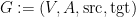
Graphs are dealt with in a slightly unusual way (for me) as quadruples $G := (V, A, \mbox{src}, \mbox{tgt})$ of a set of vertices $V$ , a set of arrows $A$ , a functions $\mbox{src}$ , $\mbox{tgt}$ mapping each arrow into its source and destination vertex. This corresponds then to what I would call a multigraph, as parallel edges can exist, though it is called a graph in the book.

For each of the structures discussed, we finish by looking at their morphisms.

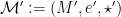
As an example, let ${\mathcal M} := (M, e, \star)$ and ${\mathcal M'} := (M', e', \star')$ be monoids (the tuple is of the set, identity element, and operation). Then a monoid homomorphism $f: {\mathcal M} \to {\mathcal M'}$ is a function $f: M \to M'$ preserving identity and operation, i.e. (i) $f(e) = e'$ and $f(m_1 \star m_2) = f(m_1) \star' f(m_2)$ for all $m_1, m_2 \in M$ .

Similarly, for graphs, graph homomorphisms $f: G \to G'$ for $G := (V, A, \mbox{src}, \mbox{tgt})$ and $G' := (V', A', \mbox{src}', \mbox{tgt}')$ are defined as pairs of functions $f_0: V \to V'$ and $f_1: A \to A'$ preserving the endpoints of arrows, i.e. such that the diagrams below commute.

Order morphisms are similarly defined, this time as those preserving order.

Thus we are introduced to several different (somewhat) familiar mathematical structures, and in each case we’re learning about how to describe morphisms on these structures that somehow preserve the structure.

Categories, Functors, and Natural Transformations

Things really heat up in Chapter 5, where we actually begin to cover the meat of category theory. This is exciting and kept me hooked by the pool. The unusual presentation of certain aspects in previous chapters (e.g. the graphs) all made sense during this chapter.

A category $\mathcal{C}$ is defined as a collection of various things: a set of objects $\text{Ob}(\mathcal{C})$ , a set of morphisms $\text{Hom}_{\mathcal{C}}(x,y)$ for every pair of objects $x$ and $y$ , a specified identity morphism $\text{id}_x$ for every object $x$ , and compositions $\circ: \text{Hom}_{\mathcal{C}}(y,z) \times \text{Hom}_{\mathcal{C}}(x,y) \to \text{Hom}_{\mathcal{C}}(x,z)$ . To qualify as a category, such things must satisfy identity laws and also associativity of composition.

Examples of the category of Monoids, of Groups, of Sets, of Graphs, of Pre-Orders, etc., are explored. Isomorphisms between objects in a category are carefully defined.

Functors are introduced as transformations from one category to another, via a function transforming objects and a function transforming morphisms, such that identities and composition and preserved. Functors are then used to rigorously explore the connections between preorders, graphs, and categories, and I finally understood why the author had focused so much on preorders in the previous chapters!

Things started to take a surprising and exciting turn for me when the author shows, via the use of functors, that a monoid is a category with one object (the set of the monoid becomes the morphisms in the category), and that groups can therefore be understood as categories with one object for which each morphism is an isomorphism. This leads to a playful discussion, out of which pops groupoids, amongst other things. Similar gymnastics lead to preorders reconstituted as categories in which hom-sets have one or fewer elements, and graphs reconstituted as functors from a certain two-object category to $\mathbf{Set}$ . Propositional logic is re-examined from a categorical perspective, though I suspect this is just scratching the surface of the interplay between category theory and logic, and I’d love to read more about this. For me, this was a highlight – that by playing with these definitions and trying things out, all these wonderful familiar structures arise.

The final part of this chapter deals with natural transformations. Just as functors transform categories to categories, natural transformations transform functors to functors. 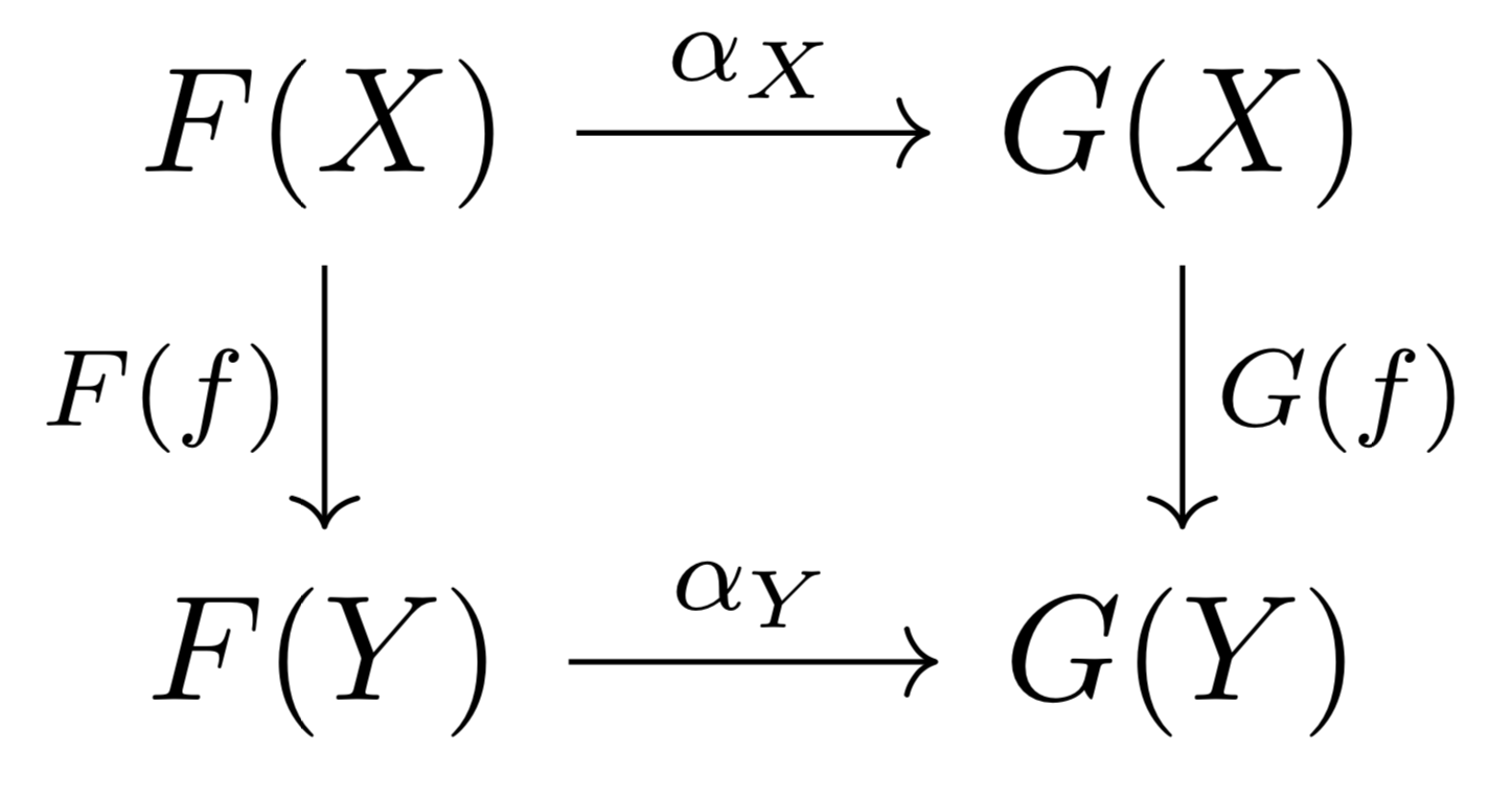Specifically, a natural transformation between functor $F : {\mathcal C} \to {\mathcal D}$ and $G : {\mathcal C} \to {\mathcal D}$ is defined as a morphism (in ${\mathcal D}$ ) $\alpha_X$ for each object $X$ in ${\mathcal C}$ , such that the diagram below commutes for every morphism $f : X \to Y$ in ${\mathcal C}$ .

Screenshot 2019-08-01 at 04.52.46

I think this section on natural transformations is where the huge number of exercises in the book really came into its own; I doubt very much I would’ve grasped some of the subtleties of natural transformations without them.

We learn about two kinds of composition of natural transformations. The first combines two natural transformations on functors $F,G,H : {\mathcal C} \to {\mathcal D}$ , say one $\alpha: F \to G$ and one $\beta: G \to H$ to obtain a natural transformation $\beta \circ \alpha: F \to H$ . The other combines a natural transformation $\gamma_1$ between functors $F_1, F_2 : {\mathcal C} \to {\mathcal D}$ with one $\gamma_2$ between functors $G_1, G_2 : {\mathcal D} \to {\mathcal E}$ , to produce one, $\gamma_2 \Diamond \gamma_1: G_1 \circ F_1 \to G_2 \circ F_2$ .

An equivalence relation ${\mathcal C}' \simeq {\mathcal C}$ – weaker than isomorphism – is introduced on categories as a functor $F : {\mathcal C} \to {\mathcal C}'$ such that there exists a functor $F' : {\mathcal C}' \to {\mathcal C}$ and natural isomorphisms $id_{\mathcal C} \xrightarrow{\cong} F' \circ F$ and $id_{{\mathcal C}'} \xrightarrow{\cong} F \circ F'$ . This seemed odd to me — the lack of insistence on isomorphism for equivalence — but the examples all make sense. More importantly it is shown that this requirement is sufficient for the on-homomorphism part of the functor $F$ to be bijective for every fixed pair of objects in ${\mathcal C}$ , which feels right. I think my understanding could benefit from further interesting examples of usefully equivalent but non-isomorphic categories though – suggestions welcome!

Limits and Colimits

Chapter 6 is primarily given over to the definitions and discussion of limits and colimits, generalising the ideas in $\mathbf{Set}$ to other categories. The chapter begins by looking again at product and coproduct. As an example, for a category ${\mathcal C}$ , with objects $X, Y \in \text{Ob}({\mathcal C})$ , a span is defined as a triple $(Z, p, q)$ where $Z$ is an object in ${\mathcal C}$ and $p : Z \to X$ and $q : Z \to Y$ are morphisms in ${\mathcal C}$ . A product $X \times Y$ is then defined as as span on $X$ and $Y$ such that for any other span $(Z, p, q)$ on $X$ and $Y$ , there exists a unique morphism $t_{p,q}$ such that the following diagram commutes. 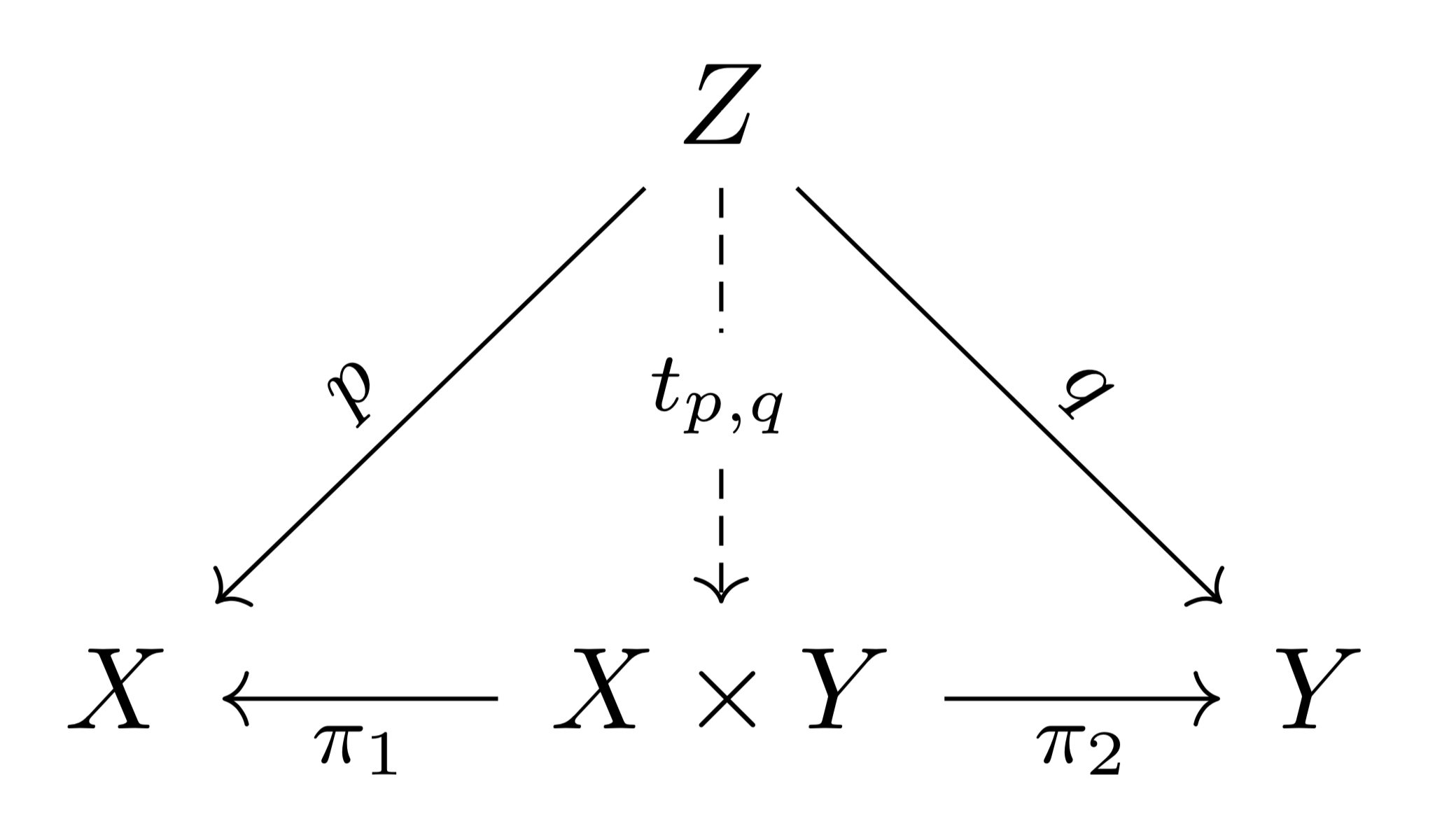Again, I rather like the author’s slogan for this: “none shall map to $X$ and $Y$ except through me!”

Screenshot 2019-10-06 at 15.36.29

The chapter then further generalises these ideas to the the ideas of limit and colimit. This section was a step up in abstraction and also one of the least “applied” parts of the book. It has certainly piqued my interest – what are limits and colimits in various structures I might use / encounter in my work? – but I found the examples here fairly limited and abstract compared to the copious ones in previous chapters. It’s in this chapter that universal properties begin to rear their head in a major way, and again I’m still not totally intuitively comfortable with this idea – I can crank the handle and answer the exercises, but I don’t feel like I’m yet at home with the idea of universal properties.

Categories at Work

In the final section of the book, we first study adjunctions. Given categories ${\mathcal B}$ and ${\mathcal A}$ , an adjunction is defined as a pair of functors $L: {\mathcal B} \to {\mathcal A}$ and $R: {\mathcal A} \to {\mathcal B}$ together with a natural isomorphism $\alpha$ whose component for $A \in \text{Ob}({\mathcal A})$ , $B \in \text{Ob}({\mathcal B})$ is $\alpha_{B,A}: \text{Hom}_{\mathcal A}(L(B), A) \xrightarrow{\cong} \text{Hom}_{\mathcal B}(B, R(A))$ . Several preceding results and examples can then be re-expressed in this framework, and understood as examples of adjunctions. Adjuctions are also revisited later in the chapter to show a close link with monads.

Categories of functors are discussed, leading up to a discussion of the Yoneda lemma. This is really interesting stuff, as it seems to cross huge boundaries of abstraction. Consider a category ${\mathcal C}$ . Spivak first defines a functor $Y_c := \text{Hom}_{\mathcal{C}}(c, -) : {\mathcal C} \to \mathbf{Set}$ sending objects in ${\mathcal C}$ to the set $\text{Hom}_{\mathcal C}(c,d)$ and similarly for morphisms. This is then used in the following theorem:

Let ${\mathcal C}$ be a category, $c \in \text{Ob}(\mathcal{C})$ be an object, and $I: {\mathcal C} \to \mathbf{Set}$ be a set-valued functor. There is a natural bijection $\text{Hom}_{\mathcal{C}-\mathbf{Set}}(Y_c, I) \xrightarrow{\cong} I(c)$ .

This looks super weird: the right-hand side is just a plain old set and yet the left hand-side seems to be some tower of abstraction. I worked through a couple of examples I dreamt up, namely $\mathcal{C} = \mathbf{1}$ (the category with one object) with $I$ mapping that object to an arbitrary set, and $\mathcal{C} = \mathbf{Set}$ with $I = \text{id}_{\mathbf{Set}}$ and convinced myself this works just fine for those two examples. Unfortunately, the general proof is not covered in the book – readers are referred to Mac Lane – and while some discussion is provided regarding links to databases, I felt like I need a proof to properly grasp what’s going on here under the hood.

Monads are then covered. I’ve briefly seen monads in a very practical context of functional programming, specifically for dealing with I/O in Haskell, but I’ve never looked at them from a theoretical perspective before.

A monad on $\mathbf{Set}$ (monads are only defined in the book on $\mathbf{Set}$ , for reasons not totally apparent to me) is defined as a triple $(T, \eta, \mu)$ consisting of a functor $T: \mathbf{Set} \to \mathbf{Set}$ , a natural transformation $\eta: \text{id}_{\mathbf{Set}} \to T$ , and natural transformation $\mu: T \circ T \to T$ such that the following diagrams commute:

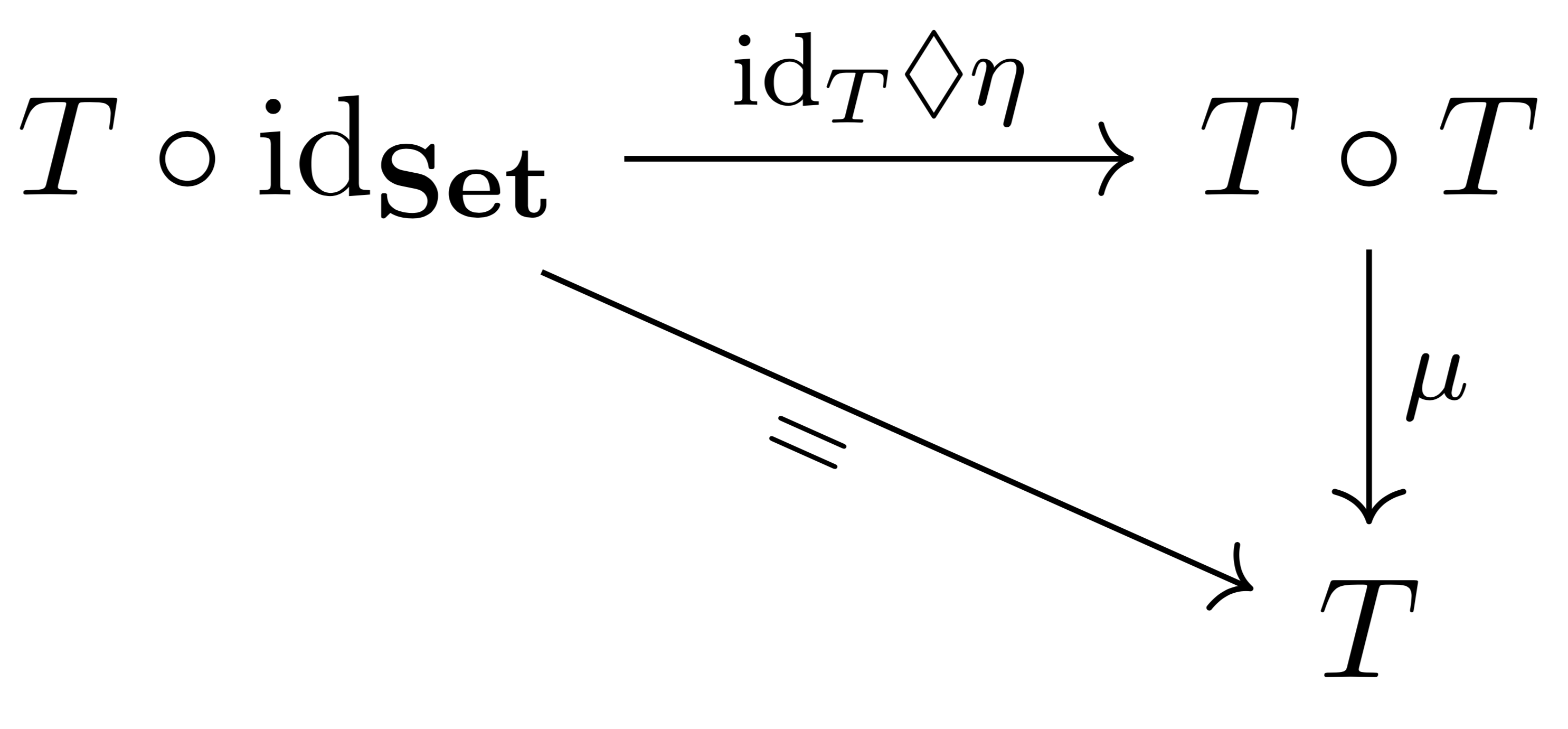
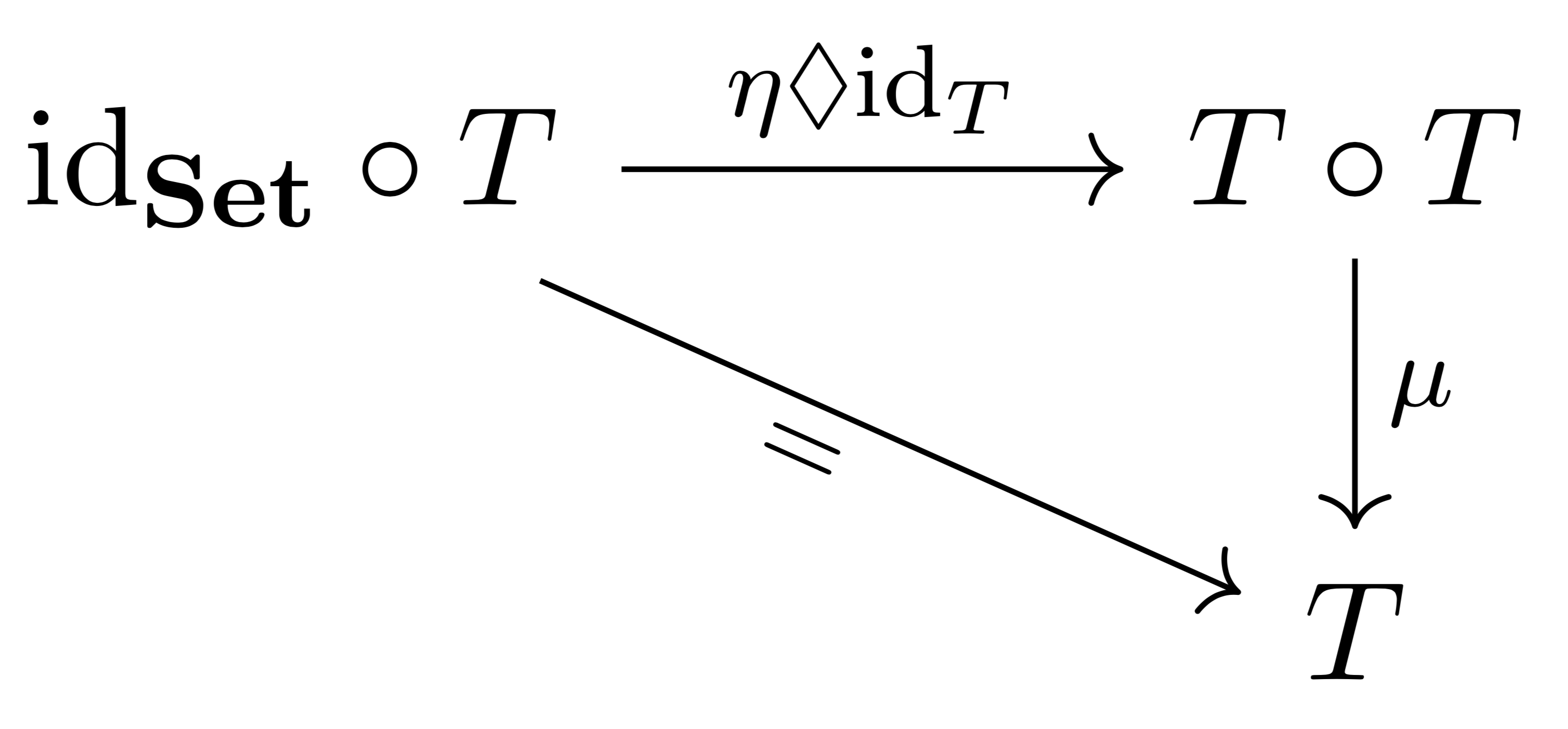
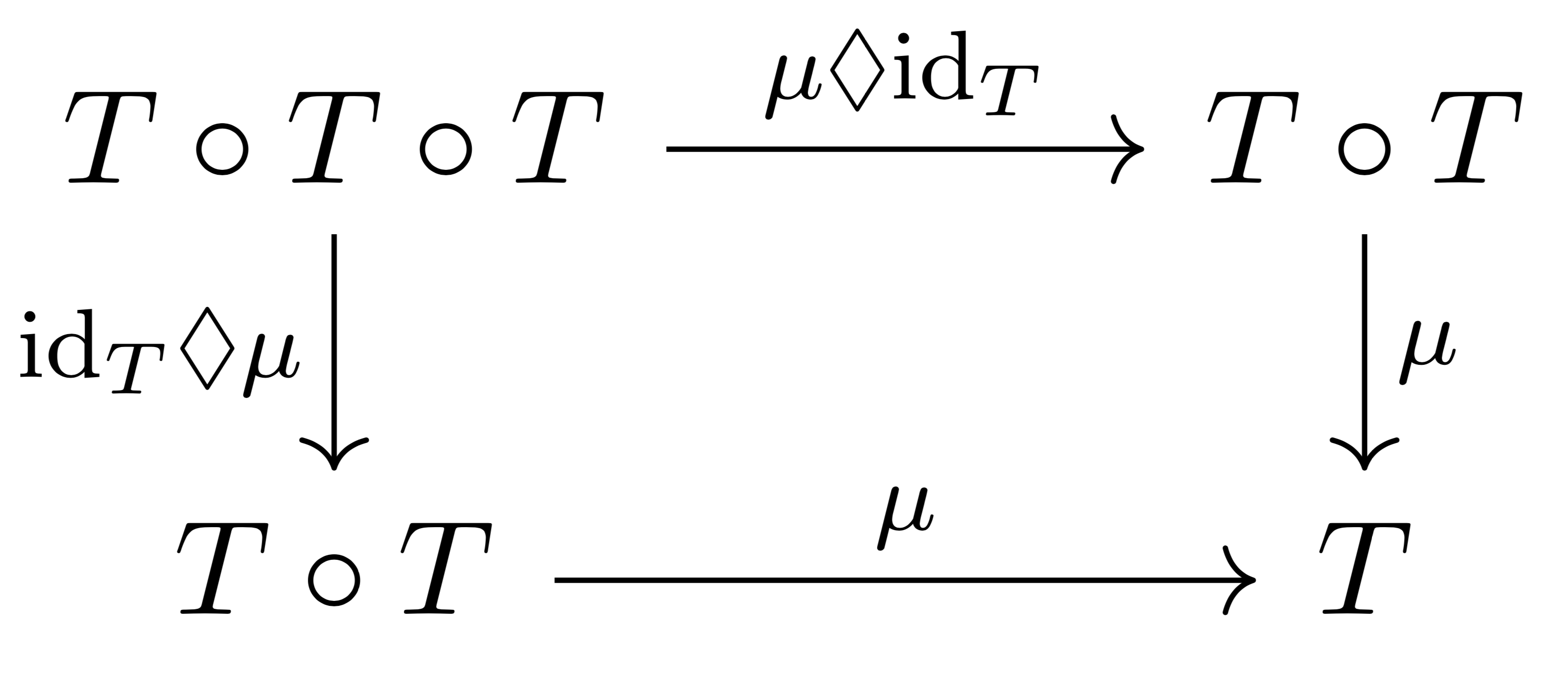
Screenshot 2019-12-08 at 14.52.30

I found this discussion enlightening and relatively straight-forward. Firstly, exception monads are discussed, like Maybe in Haskell, and a nice example of wrapping sets and their functions into power sets and their functions, for which I again enjoyed the exercises. Kleisli categories of monads are defined, and it then becomes apparent why this is such a powerful formalism to think about concepts like program state and I/O.

The Kleisli category $\mathbf{Kls}(\mathcal{T})$ of a monad $\mathcal{T} = (T, \eta, \mu)$ on $\mathbf{Set}$ is defined as a category with objects $\text{Ob}(\mathbf{Kls}(\mathcal{T}) = \text{Ob}(\mathbf{Set})$ and morphisms $\text{Hom}_{\mathbf{Kls}(\mathcal{T})}(X,Y) = \text{Hom}_{\mathbf{Set}}(X,T(Y))$ . Identity is $\text{id}_X: X \to X$ in $\mathbf{Kls}(\mathcal{T})$ is exactly $\eta_X$ in $\mathbf{Set}$ and composition of morphisms $f: X \to Y$ and $g: Y \to Z$ in $\mathbf{Kls}(\mathcal{T})$ is given by $\mu_z \circ T(g) \circ f$ in $\mathbf{Set}$ . You can intuitively see the ‘baggage’ of $T$ being carried through in $\mathbf{Set}$ yet hidden from view in $\mathbf{Kls}$ .

Finally, the book ends with a (very) brief discussion of operads. I’ve not come across operads before, and from this brief discussion I’m not really sure what they ‘buy’ me beyond monoidal categories.

General

The exercises are copious and great, especially in the earlier chapters. They kept me engaged throughout and helped me to really understand what I was reading, rather than just think I had. In the later exercises there are many special cases that turn out to be more familiar things. This is both enlightening “oh, an X is just a Y!” and frustrating “yeah, but I want to see Xs that aren’t Ys, otherwise what’s this all heavyweight general machinery for?” I guess this comes from trying to cover a lot of ground in one textbook.

I am struck by just how much mental gymnastics I feel I had to go through to see mathematical structures from the “outside in” as well as from the “inside out”, and how category theory helped me do that. This is a pleasing feeling.

The slogans are great and often amusing, e.g. when describing a functor from the category of Monoids to the category of Sets, “you can use a smartphone as a paperweight.”

The book ends rather abruptly after the brief discussion of operads, with no conclusion. I felt it would be nice to have a summary discussion, and perhaps point out the current directions the field of applied category theory is taking.

Overall, this book has been an enlightening read. It has helped me to see the commonality behind several disparate mathematical structures, and has encouraged me to look for such commonality and relationships in my own future work. Recommended!

Review: Verified Functional Programming in Agda

Agda is a dependently typed programming language. I’ve read about dependent types on and off for the past few years in magazine articles as well as discussed them a little with my collaborator Dan Ghica and others, but never really had the time to properly experiment until this Easter holiday. This book – by Aaron Stump – is interesting because it’s basic, practical, and jumps right into coding. I thought it would be good for someone like me who wants to play with the practice of dependent types and only delve into theoretical concerns as necessary or motivated to do so.

The book comes with its own Agda library, the Iowa Agda Library (IAL), a basic library of Booleans, lists, etc., simply written for the beginner to understand. It has a lot of exercises and code snippets based on that library which I found useful and relatively easy to follow.

The book assumes no functional programming expertise, and since I’ve done a (very) little bit of functional programming in Haskell in the distant past, this made the introductory material easy to follow and a useful revision aid.

Introductory Agda

The early parts of the book – Chapters 1 to 4 – are based on various data structures: Booleans, natural numbers, lists. Here the functional programming adds little to what I’ve seen before. The neat thing is the ability to use Agda as a theorem prover. This is what is described in the book as “external verification” – you write code and then you prove – separately – theorems about the code.

Firstly, let’s take a look at some example Agda code, taken from Chapter 4:


take : ∀{ℓ}{A : Set ℓ} → (n : ℕ) → 𝕃 A → 𝕃 A
take 0       _         = []
take (suc n) []        = []
take (suc n) (x :: xs) = x :: take n xs

There’s a few interesting things here already. Firstly, unicode! It feels surprisingly liberating to write unicode characters in code. Secondly the type declaration declares (via ∀), the function to be polymorphic – it operates on lists (𝕃 from IAL) of any type A (of any level ℓ within a hierarchy of type levels).

The real excitement comes when we start proving theorems. For example, given the function nthTail from IAL which returns all elements after the first n elements in a list (and the empty list if the list has fewer than n elements), we can write


ex46 : ∀{ℓ}{A : Set ℓ} (n : ℕ)(l : 𝕃 A) → (take n l) ++ (nthTail n l) ≡ l
ex46 0        _                           = refl
ex46 (suc n) []                           = refl
ex46 (suc n)  (x :: xs) rewrite ex46 n xs = refl

Here ex46 is just the name of my proof (it was Exercise 4.6 in the book). The type declaration for the function ex46 can be read as “I’ll produce a proof that concatenating (take n l) with (nthTail n l) just produces l for all natural numbers n and for all lists of elements of any type A. Here ≡, taken from IAL, is propositional equality, and the only property of it we’re using is reflexivity; in fact the only inhabitant of this type is refl. The first two lines of the proof work because the definitions of take and nthTail are such that when the first argument is zero or the second argument is empty, the left and right hand side normalize to the same result, namely .l ≡ .l in the first case (.l being the name assigned to the second unnamed argument _) and [] ≡ [] in the second case. The third case explicitly uses induction: rewrite is a directive that applies the induction hypothesis ex46 n xs to the proof of ex46 (suc n) (x :: xs). Very pleasing!

Dependent Types Revealed

Chapter 5 is where we really start to see the power of dependent types. Up until this point, we’ve written functional programs and then proved properties about those programs. We have definitely used dependent types in the process, but they were somehow “invisible” to us as a user, and – at least for the exercises in the book – we could ignore the dependent-type based implementation without really affecting the usability of the approach. Chapter 5 shows how the proofs can be part of the programs themselves, using the type system to express the properties we wish to enforce. The simplest and clearest example given is a declaration of a vector datatype:


data 𝕍 {ℓ} (A : Set ℓ) : ℕ → Set ℓ where
[] : 𝕍 A 0
_::_ : {n : ℕ} (x : A) (xs : 𝕍 A n) → 𝕍 A (suc n)

Note here that a vector, unlike a list, has a specific length built into its type. As a result, you get various properties for free, for example Agda’s type system verifies that the length of the concatenation of two vectors is the sum of the individual lengths from a straight-forward definition of a concatenation operation; the code below type checks, and that’s all that necessary.


_++𝕍_ ∀{ℓ}{A : Set ℓ}{n m : ℕ} → 𝕍 A n → 𝕍 A m → 𝕍 A (n + m)
[] ++𝕍 ys = ys
(x :: xs) ++𝕍 ys = x :: (xs ++𝕍 ys)

A more complex example of Braun trees is described in detail in the book. These are binary trees where the data at a node has a value less than or equal to that of its children while the size of the node left and right subtrees are either equal or the left subtree is exactly one node larger than the right subtree. The author chooses to encode this latter property within the declaration of the Braun tree type, and then shows how to write code for tree insertion, deletion, etc.

I enjoyed this chapter, though it had me puzzling for quite some time over sigma types, a subtle and powerful idea that I think deserves a bit more discussion than the space given in the book; I ended up reading around this topic a bit before I felt comfortable. An example given considers a function that turns lists into vectors. Immediately we have a problem – what is the return type of this function? It should be (𝕍 A n) but n is not fixed! The solution presented is to return a type written in Agda as Σ ℕ (λ n → 𝕍 A n); an inhabitant of this type should be interpreted as “a pair consisting of a natural number and a function which, when applied to that natural number, returns the vector type we’re actually interested in.” This takes a little getting used to!

Type-Level Computation

Chapter 6, introduces the idea of proof by reflection, amongst other things. This looks super-powerful, and I’m motivated to dig further into this topic when I have the time. The author illustrates the concept by creating a list simplifier, which simplifies expressions on lists. By reflecting the operations on lists as corresponding constructors for list expressions, and then proving the soundness of the simplifier, he is able to use this soundness proof to, inter alia, prove properties about the operations operating on lists. The example is really interesting, though unlike in previous chapters of the book, it’s not really discussed in detail in Chapter 6, and you have to look carefully at the code accompanying the book to see how it all fits together.

The other primary example of Chapter 6 is a statically typed version of printf, the archetypal type-evasive function of my youth

int printf( const char *restrict format, ... );

Here, the author presents an example credited to Augustsson, showing that dependent types can come to the rescue essentially by providing a type for C’s “…” which depends on the format string.

The integer example from this chapter is the closest to my own interests, showing how integers can be defined using naturals in an interesting way: an integer is a natural together with a sign which is unit (trivial) if the natural is zero but has Boolean type otherwise, i.e. the type of the sign is dependent on the value of the natural, leading to the following type declaration and definition of ℤ [taken from here].


ℤ-pos-t : ℕ → Set
ℤ-pos-t 0 = ⊤
ℤ-pos-t (suc _) = 𝔹

data ℤ : Set where
mkℤ : (n : ℕ) → ℤ-pos-t n → ℤ

I had followed through the discussion in the book easily, but came totally unstuck when trying to implement a seemingly obvious exercise I set myself: prove that integer multiplication commutes using a pre-existing proof of the commutativity of multiplication over the naturals.

I had defined integer multiplication as:


_*ℤ_ : ℤ → ℤ → ℤ
_*ℤ_ (mkℤ 0 _)        _                = mkℤ 0 triv
_*ℤ_ (mkℤ (suc n) _)  (mkℤ 0 _)        = mkℤ 0 triv
_*ℤ_ (mkℤ (suc n) sn) (mkℤ (suc m) sm) = mkℤ ((suc n) * (suc m)) (sn xor sm)

where triv is the single inhabitant of the ⊤ type. I had therefore naively assumed that one could simply write the proof as:

*ℤcommutes (mkℤ 0 _)        (mkℤ 0 _) = refl
*ℤcommutes (mkℤ 0 _) (mkℤ (suc bN) _) = refl
*ℤcommutes (mkℤ (suc aN) _) (mkℤ 0 _) = refl
*ℤcommutes (mkℤ (suc a) sa) (mkℤ (suc b) sb) rewrite xor-comm sa sb | (*comm (suc a) (suc b)) = refl

However, this fails – for the final pattern – for a very interesting reason that was, however, totally incomprehensible to me at first. Agda reports:

𝔹 !=< ℤ-pos-t w of type Set
when checking that the type
(b a w : ℕ) →
w ≡ suc (a + b * suc a) →
(sa sb : 𝔹) →
mkℤ w (sb xor sa) ≡ mkℤ (suc (a + b * suc a)) (sb xor sa)
of the generated with function is well-formed

“Huh? ‘Generated with function?'”

Thus began a small odyssey of Easter holiday evenings spent learning how rewrites are implemented as withs, and how withs in turn are implemented using generated auxiliary functions. I found Norrell and Chapman’s tutorial, together with the good quality documentation provided me with the necessary additional background required to teach myself what was going on here and to produce a final, working proof:


*ℤcommutes : ∀ (a b : ℤ) → a *ℤ b ≡ b *ℤ a
*ℤcommutes (mkℤ 0 _)        (mkℤ 0 _)        = refl
*ℤcommutes (mkℤ 0 _)        (mkℤ (suc m) sm) = refl
*ℤcommutes (mkℤ (suc n) _)  (mkℤ 0 _)        = refl
*ℤcommutes (mkℤ (suc n) sn) (mkℤ (suc m) sm)
with m + n * suc m | *comm (suc n) (suc m)
... | .(n + m * suc n) | refl rewrite xor-comm sn sm = refl

I have mixed feelings about this experience. On the one hand, I’ve learnt a lot about Agda specifically (and dependent types in general) by being forced to go through this process to understand what’s going on under the hood. On the other hand, this seems like a lot of hoops to jump through for this simple proof, and the book under review didn’t have all the answers I was looking for to solve the exercise. I don’t see the latter point as a big deal, but if you’re going to do your explorations on holiday, make sure you have a wifi connection available so you can look beyond the book for help!

Selected Topics

The remainder of the book is eclectic but interesting.

Chapters 7 and 8 combine to produce a larger example piece of code – a Huffman coder / decoder. It’s good to see the ideas put into practice in a larger case study, of course, though these chapters were less interesting to me personally.

Chapter 9 really recaptured my attention, though! The author uses Agda’s types to reason about termination. He explicitly sets up a general datatype representing what it means for a relation DAG to not have any infinite chain of successor nodes starting from a given named node, something he calls a terminating relation. He then proves in Agda that > over ℕ is terminating in this sense. The chapter then goes on to apply this to producing a termination proof for a recursively defined division function. I’m aware of this kind of reasoning, and have even played a bit with tools making use of these ideas like Byron Cook et al.‘s Terminator. So it’s interesting to see this in the context of the type system of Agda where in fact it becomes rather important since all functions must terminate in Agda – otherwise none of the proofs discussed above make sense!

The final chapter of the book, Chapter 10, formalises some ideas in a particular logic within Agda, using Agda to prove soundness and completeness of the logic.

Conclusion

The book ends rather abruptly with Chapter 10 on intuitionistic logic and Kripke semantics. There is no rounding off, summarising lessons learnt or directions for future research or indeed practical programming advice.

Nevertheless, I learnt a lot from reading this book – and a lot more from doing its exercises! It’s given me an initial understanding of one of the most recently talked-about developments in programming. I’m left keen to try to apply this to some real-world problems in my research! Well recommended holiday reading.

Book Review: Complexity and Real Computation

Over several holiday and train journeys, I’ve been slowly reading and digesting this book by Blum, Cucker, Shub, and Smale. It’s one of a number of books I’ve read that are definitively not in my research field – hence holiday reading – and yet touches it tangentially enough to get me excited. I’ve been interested in computation defined in terms of real numbers ever since my own PhD thesis back in 1998-2001, which looked at ways to take a specific class of computation defined on the reals and synthesise hardware circuits operating in very efficient fixed-point arithmetic. While my own work has often involved specifying computation on the reals, including recently exploiting the differences between real and finite precision computation for circuits, this book takes a fundamental look at computation over the reals themselves. In particular, it looks at what happens to notions of computability and complexity if you consider real addition, multiplication, division, and subtraction as basic operators in a computation model: what is computable, what resulting complexity bounds can be proved? Ever since my first exposure to algebraic geometry, especially real algebraic geometry, I see it everywhere – and have even made some small forays [1,2] into harnessing its power for hardware design. It’s a delight to see computability and algebraic geometry coming together so neatly in this text.

Part I: Basic Development

The authors define a computational model that is very natural for analysis: a computation consists of a control-flow graph consisting of input nodes, computation nodes (polynomial or rational maps), branch nodes (checking for equality or inequality, depending on whether the ring / field being computed over is ordered), and output nodes. For the remainder of this review, I will consider only computation over the reals, though some of the results are more general. Theorems naturally flow from this setting. My favourites: the halting set of a machine is a countable union of semialgebraic sets; there are “small” systems of polynomial inequalities, of low degree, describing behaviour of a machine up to $T$ time steps. As a by product, the first practical uses of this theory are illustrated, e.g. a proof that the Mandelbrot set is not decidable over ${\mathbb R}$ . The interplay between the uncountable (program state) and the countable (program counter state) leads to some intricate and enjoyable analysis.

Chapter 3 generalises classical results for universal Turing machines, typically expressed in terms of unbounded tapes with binary storage at each location, to the case where an element of an arbitrary ring is stored at each location (imagine a real number stored at each location). Additional shift operations are introduced to deal with moving along the tape. It is shown that operation over unbounded sequences allows for uniformity of algorithm across dimensionality but does not add additional computational power for fixed dimensionality. In finite time we can only explore a finite portion of the tape, so we still retain the semi-algebraic (or countable union of semi-algebraic) sets for the halting sets derived in Chapter 2.

Chapter 4 extends the usual complexity-theoretic classes P and EXP to computation over a ring. Computation over ${\mathbb Z}_2$ corresponds to the classical case. There are no great surprises here for a reader who has read a basic text in computational complexity together with Chapters 1-3 of this book. The authors round off the chapter by using this new machinery to cast results from Goedel and Tarski from an interesting perspective. For example, Goedel becomes there exist definable undecidable sets over ${\mathbb Z}$ , while Tarski becomes every definable set over ${\mathbb R}$ is decidable over ${\mathbb R}$ . Questions of definability are then put off until the very end of this book – and this review.

Chapter 5 shows how classical NP, NP-complete and NP-hard definitions carry forward into computation over a general ring. Then, specialising the results to particular rings and particular costs of elementary operations (unit? dependent on size of numbers?), the NP-completeness of various key problems are shown. In particular, it is shown that the classical 3-SAT NP-completeness result can be obtained by working over the ring ${\mathbb Z}_2$ . The chapter ends with an interesting discussion of the P ?= NP question over various rings and with various costs. It’s interesting, for example, that the problem of determining whether there is a zero of a degree-4 polynomial is NP-complete over ${\mathbb R}$ while that of a degree 3 is in P; analogous to the situation with 3-SAT versus 2-SAT in the classical setting.

Chapter 6 moves on to look specifically at machines over ${\mathbb Z}$ with bit cost, i.e. the bigger the number, the more it costs to operate on it. It is shown that these machines are polynomially equivalent to those operating over ${\mathbb Z}_2$ with unit cost, i.e. anything you can write in terms of algebraic operations over ${\mathbb Z}$ you can also write under the classical Turing model of computation, and vice versa, with only polynomial blow up in execution steps. This is not too surprising, and ultimately derives from the standard possibility of writing an integer as its binary expansion. The chapter then takes a detour via Farkas’s Lemma to show that linear programming feasibility (LPF) is in NP, a rather intricate result I first saw in Schrijver’s encyclopaedic book when working with my former PhD student Qiang Liu on discrete linear algebra for hardware memory optimization. It is noted that LPF’s status depends strongly on the choice of computation model and ring: in the (equivalent) classic setting of integers with bit cost it is NP-complete, over rationals with bit cost it is in P, while its status over ${\mathbb R}$ is apparently open.

Part II: Some Geometry of Numerical Algorithms

This part of the book turns to look at specific algorithms such as Newton’s method and a homotopy method for nonlinear optimization. In each case, complexity results are given in terms of the number of basic real arithmetic operations required. Some fun analysis and quite a clear exposition of homotopy methods, which I’ve worked with before in the context of convex optimization, especially when using barrier methods for linear and convex quadratic programming, something I looked at quite carefully when trying to design FPGA-based computer architectures for this purpose.

The chapter on Bézout’s Theorem assumed a rather more thorough grounding in differential topology than I have, and I wasn’t entirely sure how it sat with the rest of the work, as the constructive / algorithmic content of the theorems was less apparent to me.

The final chapters of this part of the book took me back to more familiar territory – first introduced to me by the outstandingly clear encyclopaedic textbook by Nick Higham – the discussion of condition numbers for linear equations and the relationship to the loss of precision induced by solving such systems (roughly, the relative error in the right hand side of $Ax = b$ gets amplified by the condition number of the matrix $A$ ). What was interesting here is the authors’ probabilistic analysis – looking at the expected condition number if the matrix elements are iid Gaussian variables, for example. I have skimmed another book also co-authored by Cucker – on this very topic, and I’m waiting to have the time to read it. Condition for polynomial problems is covered, leading to complexity results for logarithmic barrier interior point methods for linear equations over $\mathbb{Q}$ (spoiler: it’s in $\mathbb{P}$ ).

Part III: Complexity Classes over the Reals

After Part II, which was only interesting to me in parts, I started to get excited again by Part III. Lower bounds on the computational complexity of various problem are derived here based on some very interesting ideas. The basic scheme is to bound the number of different connected components in a (semi-)algebraic set in terms of the degree of the polynomials and the number of variables involved. The number of different connected components can then be used to bound the number of steps an (algebraic) machine takes to decide membership of that set.

In Chapter 17, the framework is extended to probabilistic machines, and the standard definition of BPP is extended to computation over an arbitrary ring, giving $BPP_{R}$ . The chapter then goes on to show that probabilistic machines over $\mathbb{R}$ can be simulated by deterministic machines over $\mathbb{R}$ without blowing up execution time, i.e. that $P_\mathbb{R} = BPP_\mathbb{R}$ , whereas this is unknown for the classical setting. The essence of the argument makes use of a special real number (shown, non constructively, to exist), encoding all the different “coin flips” that a probabilistic program makes during its execution, which is then encoded as a machine constant in the simulating machine.

Parallelism – close to my heart – is covered in Chapter 18, through the introduction of complexity classes $PL^k_\mathbb{R}$ , parallel polylogarithmic time, for sets that can be decided in time $O(\log^k n)$ using a polynomial number of processors, and $PAR_\mathbb{R}$ , parallel polynomial time, for sets that can be decided in polynomial time using an exponential number of processors (definitions following a SPMD computational model). Algorithms are derived for matrix inversion and product and a result is cited for parallel quantifier elimination over the reals.

Chapter 22 looks at the relative power of machines over $\mathbb{Z}_2$ , i.e. the classical model, compared to real machines which take inputs restricted to be drawn from $\{0,1\}$ . It’s fairly obvious that the latter setting can provide a lot of additional power, for example deciding membership of a set in $\mathbb{Z}^\infty_2$ can be done by encoding the characteristic function of the set as the digits of some real constant in the program. It is then shown that additive real machines (a restricted form of the machines discussed above, containing no multiplication or division) that additionally contain branching only on equality can solve exactly the same problems in polynomial time as in the classical model. This is unlike the case where branching can be over inequality, where some additional computational power is provided by this model.

Descriptive Complexity, Chapter 23 is interesting: the descriptive power of (a particular) first order logic extended with fixed point and maximisation operations and of existential second order logic are shown to correspond to a particular subclass of $P_\mathbb{R}$ problems and $EXP_\mathbb{R}$ , respectively. In the latter case, I think this essentially says that known results in the classical case carry forward to computation over the reals despite the move away from a finite ring. I am not familiar enough with computational complexity literature to comment on how the former result compares with the classical setting, and I didn’t feel that this point is was very well described in the book.

Conclusion

Overall, I found this book a little eclectic, especially Part II, reflective of the fact that it has clearly been put together drawing from a variety of different primary sources spanning several decades. This should not be seen as a criticism. The choice of material was wonderful for me – as holiday reading at least! – tangentially touching so many different topics I’ve seen during my career and drawing me in. In places, the development was over an arbitrary ring, in places over $\mathbb{C}$ and in places over $\mathbb{R}$ , and although for some sections it was absolutely clear why, for others it was less clear. Overall, though, I would very much recommend anyone who likes to keep a foot in both the continuous and discrete worlds to take a look at this book.

Book Reviews: Popular Science

A friend recently reintroduced me to the genre of popular science – specifically, popular physics – something I had left behind in my mid teens. I remember voraciously reading the books of John Gribbin as a teenager, sitting in bed in my parents’ house thinking about black holes and quantum physics. Since then I’ve been more focused on – and interested in – my particular field.

However, following prompting, I’ve recently read two popular science books: Seven Brief Lessons on Physics by Carlo Rovelli, and A Beautiful Question by Frank Wilczek. Both are good books, though very different. The former is a brief, almost poetically written waltz through relatively, quantum physics, and more recent unification efforts – it can easily be read in a single afternoon. The second is a more weighty tome, a very personal view from a Nobel Prize winner of beauty and its embodiment in the symmetries present in nature. The chapters of the latter vary in terms of how much I enjoyed them, primarily because many I felt some had too much information not to take a mathematical approach, yet this was not forthcoming. Meanwhile the former was a joy to read because it its brevity skimmed the surface and left me wanting to dig further, specifically into ideas of quantum loop gravity and into what modern neuroscience may or may not be able to tell us about the emergence of notions of “self”.

Book Review: Essential Topology

Topology is an area of mathematics with which I have no prior experience. I guess it was felt historically that engineers don’t really need topology, and this has filtered down the generations of study. Yet I’ve always found the ideas of topology intriguing, even if I have not deeply understood them. They seem to pop up in the most wide variety of places. While running a math circle for primary school kids, we ended up discussing Euler’s Polyhedron Formula, and I realised that if I wanted to explore these ideas more deeply, I would need a proper grounding in topology. From the wonderful lectures of Tadashi Tokieda which I watch with my son, to the more theoretical end of computer science I bump up against in my day-to-day research, topology seems to be everywhere. I found this book, Essential Topology by Martin D. Crossley, while browsing in a bookshop and decided to take it on holiday as holiday reading.

As presented, the book naturally falls into three parts: an introductory section, a section on basic topology, and a section on more advanced algebraic topology. Although short, the book is written as a sequence of a good number of chapters, 11 in total, which make the material more digestible. Moreover, I found the two “interludes” between sections of the book to be a great innovation – invaluable as a mechanism for orienting my reading, providing the appropriate informal guidance about the journey on which the text was taking me.

The introductory section begins with looking at the question of continuity from a rigorous perspective, bringing in both the epsilon-delta approach to continuity with which I am familiar, and an approach based on open sets with which I was not – but which is easily generalised to functions other than from $\mathbb{R}$ to $\mathbb{R}$ . It then moves on to axiomatically defines topological spaces, some standard topologies, and bases for topologies.

The second section begins to explore some of the properties that can be proved using the equipment set up in the previous chapters: connectedness, compactness, the Hausdorff property, homeomorphisms, disjoint unions, product and quotient spaces. I enjoyed this section greatly.

The third section then goes on to discuss various more advanced topics, looking at various topological invariants that have been well studied. Some highlight for me included:

Chapter 6 discusses the idea of homotopy as an equivalence between maps: two maps $f,g: S \rightarrow T$ are homotopic iff there is a continuous function $F: S \times [0,1] \rightarrow T$ allowing for a kind of continuous deformation of one function into the other, i.e. with $F(s,0) = f(s)$ and $F(s,1) = g(s)$ . This is shown to be rather a broad equivalence, for example all continuous functions on $\mathbb{R}$ are homotopic. However, working with other topological spaces, things get quite interesting. A big part of the chapter is given over to working with circles $\mathbb{S}^1$ , where it is shown that there is a countable set of homotopy classes of functions from $\mathbb{S}^1$ to $\mathbb{S}^1$ . This is very clearly described, and I seem to remember through the mists of time some of these issues cropping up informally in the context of my control theory courses as an undergraduate (or, for that matter, fathoming ${\tt unwrap}$ in Matlab as an undergraduate!) The chapter ends with a proof of the fantastically named “Hairy ball theorem,” from which – amongst other things – it follows that at any given point in time, there’s a part of the world with zero wind speed!

Chapter 7 discusses the Euler characteristic as a topological invariant and introduces some interesting theorems. After introducing the idea of a ‘triangulable space’, it is stated that if two such spaces are homotopy equivalent then they have the same Euler number. More remarkable (to me!) is that when restricted to surfaces, it is sufficient for two such surfaces to have the same Euler number and the same orientability in order for them to be homotopy equivalent. Unfortunately, the proofs of both these results are omitted – apparently they are rather involved – references are given. I certainly appreciated the results collected in this chapter, but I found the exercises quite hard compared to other chapters, possibly partly because of the proof issue, but also because I found it hard to visualise some aspects, e.g. triangulation of a surface of genus 2, and since such surfaces had only been defined informally in the preceding chapters I could not (easily) fall back on a purely algebraic approach to the geometry. I did find it particularly interesting to see the Euler characteristic rigorously defined for a general class of spaces – the very definition in the primary math circle that had brought me to this book in the first place!

Chapter 8 discusses homotopy groups. The basic idea is that one can work with homotopy classes of maps from ${\mathbb S}^n$ , the $n$ -dimensional sphere, to a space $X$ (actually pointed homotopy classes of pointed maps, but lets keep things simple) and it turns out that these classes form a group structure: they have an identity element (constant maps), an addition operation, etc. I guess the purpose here is to bring out the topological structure of $X$ , though the special role played by ${\mathbb S}^n$ was not totally apparent to me – why is this particular space so fruitful to study? I wonder if any readers can comment on this point for me.

Chapter 9 provides an introduction to Simplicial Homology, the idea – roughly – that those combinations of simplices within a simplicial complex which ‘could’ form boundaries of other simplices but ‘do’ not, tell us something about the topology of the simplicial complex. Homology is then introduced in a different form (Singular Homology) in Chapter 10, and it is stated that the two approaches coincide for triangulable spaces.

In these latter chapters of the book, some theorems tend to be stated without proof. The author is always careful to refer to other textbooks for proof, and I guess this is a necessary aspect of trying to introduce a very large subject in a brief textbook, but for me this made them somewhat less appealing than those in the first two sections. Nevertheless, I now feel suitably armed to begin looking at the world through a more topological lens. I wonder what I will see. For now I’m off to eat a coffee cup.

Book Review: Out of the Labyrinth: Setting Mathematics Free

This book, by Kaplan and Kaplan, a husband and wife team, discusses the authors’ experience running “The Math Circle”. Given my own experience setting up and running a math circle with my wife, I was very interested in digging into this.

The introductory chapters make the authors’ perspective clear: mathematics is something for kids to enjoy and create independently, together, with guides but not with instructors. The following quote gets across their view on the difference between this approach and their perception of “school maths”:

Now math serves that purpose in many schools: your task is to try to follow rules that make sense, perhaps, to some higher beings; and in the end to accept your failure with humbled pride. As you limp off with your aching mind and bruised soul, you know that nothing in later life will ever be as difficult.

What a perverse fate for one of our kind’s greatest triumphs! Think how absurd it would be were music treated this way (for math and music are both excursions into sensuous structure): suffer through playing your scales, and when you’re an adult you’ll never have to listen to music again.

I find the authors’ perspective on mathematics education, and their anti-competitive emphasis, appealing. Later in the book, when discussing competition, Math Olympiads, etc., they note two standard arguments in favour of competition: that mathematics provides an outlet for adolescent competitive instinct and – more perniciously – that mathematics is not enjoyable, but since competition is enjoyable, competition is a way to gain a hearing for mathematics. Both perspectives are roundly rejected by the authors, and in any case are very far removed from the reality of mathematics research. I find the latter of the two perspectives arises sometimes in primary school education in England, and I find it equally distressing. There is a third argument, though, which is that some children who don’t naturally excel at competitive sports do excel in mathematics, and competitions provide a route for them to be winners. There appears to be a tension here which is not really explored in the book; my inclination would be that mathematics as competition diminishes mathematics, and that should competition for be needed for self-esteem, one can always find some competitive strategy game where mathematical thought processes can be used to good effect. However, exogenous reward structures, I am told by my teacher friends, can sometimes be a prelude to endogenous rewards in less mature pupils. This is an area of psychology that interests me, and I’d be very keen to read any papers readers could suggest on the topic.

The first part of the book offers the reader a detailed (and sometimes repetitive) view of the authors’ understanding of what it means to do mathematics and to learn mathematics, peppered with very useful and interesting anecdotes from their math circle. The authors take the reader through the process of doing mathematics: analysing a problem, breaking it down, generalising, insight, and describe the process of mathematics hidden behind theorems on a page. They are insistent that the only requirement to be a mathematician is to be human, and that by developing analytical thinking skills, anyone can tackle mathematical problems, a mathematics for The Growth Mindset if you will. In the math circles run by the authors, children create and use their own definitions and theorems – you can see some examples of this from my math circle here, and from their math circles here.

I can’t say I share the authors’ view of the lack of beauty of common mathematical notation, explored in Chapter 5. As a child, I fell in love with the square root symbol, and later with the integral, as extremely elegant forms of notation – I can even remember practising them so they looked particularly beautiful. This is clearly not a view held by the authors! However, the main point they were making: that notation invented by the children, will be owned and understood by the children, is a point well made. One anecdote made me laugh out loud: a child who invented the symbol “w” to stand for the unknown in an equation because the letter ‘w’ looks like a person shrugging, as if to say “I don’t know!”

In Chapter 6, the authors begin to explore the very different ways that mathematics has been taught in schools: ‘learning stuff’ versus ‘doing stuff’, emphasis on theorem or emphasis on proof, math circles in the Soviet Union, competitive versus collaborative, etc. In England, in my view the Government has been slowly shifting the emphasis of primary school mathematics towards ‘learning stuff,’ which cuts against the approach taken by the authors. The recent announcement by the Government on times tables is a case in point. To quote the authors, “in math, the need to memorize testifies to not understanding.”

Chapter 7 is devoted to trying to understand how mathematicians think, with the idea that everyone should be exposed to this interesting thought process. An understanding of how mathematicians think (generally accepted to be quite different to the way they write) is a very interesting topic. Unfortunately, I found the language overblown here, for example:

Instead of evoking an “unconscious,” with its inaccessible turnings, this explanation calls up a layered consciousness, the old arena of thought made into a stable locale that the newer one surrounds with a relational, dynamic context – which in its turn will contract and be netted into higher-order relations.

I think this is simply arguing for mathematical epistemology as akin to – in programming terms – summarizing functions by their pre and post conditions. I think. Though I can’t be sure what a “stable locale” or a “static” context would be, what “contraction” means, or how “higher order relations” might differ from “first order” ones in this context. Despite the writing not being to my taste, interesting questions are still raised regarding the nature of mathematical thought and how the human mind makes deductive discoveries. This is often contrasted in the text to ‘mechanical’ approaches, without ever exploring the question of either artificial intelligence or automated theorem proving, which would seem to naturally arise in this context. But maybe I am just demonstrating the computing lens through which I tend to see the world.

The authors write best when discussing the functioning of their math circle, and their passion clearly comes across.

The authors provide, in Chapter 8, a fascinating discussion of the ages at which they have seen various forms of abstract mathematical reasoning emerge: generalisation of when one can move through a 5×5 grid, one step at a time, visiting each square only once, at age 5 but not 4; proof by induction at age 9 but not age 8. (The topics, again, are a far cry from England’s primary national curriculum). I have recently become interested in the question of child development in mathematics, especially with regard to number and the emergence of place value understanding, and I’d be very interested to follow up on whether there is a difference between this between the US, where the authors work, and the UK, what kind of spread is observed in both places, and how age-of-readiness for various abstractions correlates with other aspects of a child’s life experience.

Other very valuable information includes their experience on the ideal size of a math circle: 5 minimum, 10 maximum, as they expect children to end up taking on various roles “doubter, conjecturer, exemplifier, prover, and critic.” If I run a math circle again, I would like to try exploring a single topic in greater depth (the authors use ten one hour sessions) rather than a topic per session as I did last time, in order to let the children explore the mathematics at their own rate.

The final chapter of the book summarises some ideas for math circle style courses, broken down by age range. Those the authors believe can appeal to any age include Cantorian set theory and knots, while those they put off until 9-13 years old include complex numbers, solution of polynomials by radicals, and convexity – heady but exciting stuff for a nine year old!

I found this book to be a frustrating read. And yet it still provided me with inspiration and a desire to restart the math circle I was running last academic year. Whatever my beef with the way the authors present their ideas, their core love – allowing children to explore and create mathematics by themselves, in their own space and time – resonates with me deeply. It turns out that the authors run a Summer School for teachers to learn their approach, practising on kids of all ages. I think this must be some of the best maths CPD going.

Book Review: Surely You’re Joking, Mr Feynman

This Summer I had a long flight to Singapore. A few hours into long flights I tend to lose the will to read anything challenging, so I decided to return to a book I first read as a young teen when it was lent to me by family friend fred harris, the book Surely You’re Joking, Mr Feynman. I remember at the time that this book was an eye opener. Here was a Nobel prize winning physicist with a real lust for life coupled with an inherent enthusiasm for applying the scientific method to all aspects of life and a healthy lack of respect for rules and authority. As a teenager equally keen to apply the scientific method to anything and everything, and keen to work out my own ideas on authority and rules, yet somewhat lacking the personal confidence of Feynman, I found the book hugely enjoyable.

I still find the book hugely enjoyable. I was chuckling throughout – the practical jokes, the encounters with non-scientific “experts” and authority figures. However, I was also somewhat taken aback by Feynman’s attitude to women, which I found misogynistic in places, something that had totally passed me by as a teenager. Feynman’s attitudes were probably unremarkable for his time (Feynman was born in 1918) so I’m not attributing blame here, but I find it odd that I didn’t notice this in the 1980s. Googling for it now, I find commentary about this point is all over the Internet. It just goes to show how many subtleties pass children and teens by, something parents and educators would do well to remember.