In a couple of recent posts [1,2], I have been trying to reason through the geometric properties of block number formats. The basic idea is that when a group of numbers shares a scale factor, the small low-precision numbers inside the block are no longer meaningfully trying to approximate scalar magnitudes, as the scale has already taken care of much of the magnitude information. What remains is, to a significant extent, a question of direction.
This post is about a new preprint I have recently put out with Bardia Zadeh, “Direction-Preserving Number Representations”. The question we ask is “If a block scale has already taken care of magnitude, what should the scalar values inside the block look like if our aim is to preserve direction?”
That is not the usual question in computer arithmetic, and I can’t really find a historical precedent for this question in the usual places I would look (please let me know if you know others who have looked at this question from an arithmetic perspective!) We usually ask about absolute error, relative error, dynamic range, rounding behaviour, underflow, overflow, and so on. But in many modern machine learning settings, it is also natural to ask a more geometric question: how well do the values available inside a block cover the possible directions of a vector?
On the research methodology side, there is another aspect of this paper that is new for me personally. This is the first paper I have written where AI tools (namely GPT-5.4, GPT-5.5 and Aristotle) made a substantive contribution to the development of proof ideas, as well as to the Lean formalisation, which I am delighted we have open sourced. The AI tools definitely did not replace mathematical judgement or lead to a push button approach: the process still required many manual reformulations, checking, rewriting, and false starts. But it was a new and positive experience for me. In particular, the combination of exploratory AI assistance and Lean’s rock solid proof checking made for a very different style of research interaction from the one I am used to.
I will come back to Lean and AI below. First, let me describe the mathematical object we studied.
From scalar alphabets to directions
Suppose we have a finite scalar alphabet 
If a block has dimension 

But if the block also has an independent positive scale factor, then multiplying the whole vector by a positive scalar should not really change the information encoded by the low-precision elements. The scale can absorb that. What matters is the direction.
So the relevant object becomes

This is a finite set of points on the unit sphere. But these points can’t be placed arbitrarily on the sphere. The set has product structure, because each coordinate is chosen independently from the scalar alphabet.
The natural worst-case measure is the covering radius

This asks: given any true direction 

This lens changes the problem of how to select the alphabet. Instead of asking “which scalar values approximate real numbers well?”, we ask: which scalar values, when used coordinatewise, cover directions well?
You can see the two-dimensional directionality coverage of the floating-point alphabet with two exponent bits, one mantissa bit and one sign bit (E2M1), illustrated below. Each intersection of grid lines corresponds to a 2-vector with elements drawn from this alphabet. We may then find where the line between the origin and that intersection meets a circle (marked as red points). Note the non-uniform spacing around the circle: some regions are better covered than others.
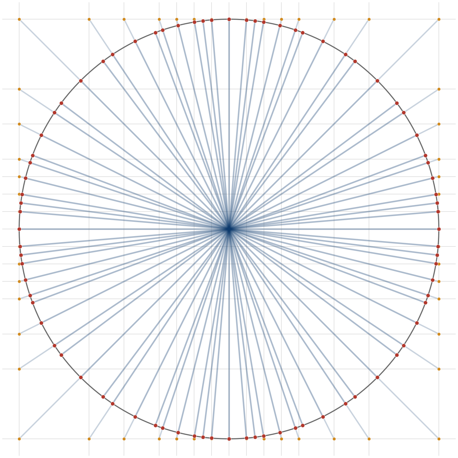
If you want to play with designing your own two-dimensional alphabet in a graphical user interface, you can get more intuition into this problem using this widget Bardia created: https://bardia01.github.io/directional_coverage_explorer/.
A Lean Interlude
As I mentioned above, I’m super pleased that we’ve open-sourced formalisations of all our theorems and definitions in Lean. The formalisation is organised so that the top-level declarations correspond closely to the paper.
The key definitions look like this:
abbrev Aq (q : Nat) : Set (Finset Real) :=
  {A : Finset Real | A.card = q}

abbrev P (n : Nat) (A : Finset Real) :
  Finset (OptimalAlphabets.SpherePoint n) :=
  OptimalAlphabets.AsymmetricProduct.asymProdSphericalCode n A

abbrev F (n : Nat) (A : Finset Real) : Real :=
  OptimalAlphabets.AsymmetricProduct.F_asym n A

abbrev rhoSph (n m : Nat) : Real :=
  OptimalAlphabets.rho_sph n m
Here Aq q is the class of scalar alphabets with 
P n A is the finite spherical code obtained by normalising nonzero elements of 
F n A is the product-code covering objective rhoSph n m is the optimal covering radius of an unconstrained spherical code with 
I’m giving these Lean definitions now so we can roughly follow along in Lean as we go for the rest of this blog post.
Product Codes versus Spherical Codes
It seems natural, almost obvious, that a product code should give worse directional coverage than a vector code chosen specifically to optimise directional coverage. Of course, the latter may not be practical, as the decoding process may be significant, but it still forms a useful baseline comparison point. Our first theoretical contribution is to quantify the gap between these two code classes.
Notice that the product structure induces a very severe geometric constraint. Even if 
The harmonic witness
A central construction in the paper is a direction that is hard for product codes to cover. Let

be the

The entries of this vector decay slowly, making the vector awkward for a finite scalar alphabet. The resulting theorem gives a lower bound on the worst-case angular error. If 

The Lean statement is compact enough to include directly:
theorem theorem2_sign_count_bound {n : Nat} (hn : 2 <= n)
    (A : Finset Real) :
  Real.arccos
    (min 1 (2 * Real.sqrt (mSign A : Real) / Real.sqrt (H n))) <=
  F n A
The notation mSign A is the Lean name for
Since 


This is a worst-case theorem. We’re not claiming that real neural network tensors look like the harmonic witness. What the theorem tells us is that if the metric is worst-case angular coverage of the entire sphere, product-structured scalar alphabets have an inherent limitation.
So What about Spherical Codes?
A product code built from a
The paper proves that, for any fixed
Here is the Lean statement:
theorem theorem4_asymptotic_strict_separation_fixed_alphabet_size
    {q : Nat} (hq : 2 <= q) :
  ∃ N : Nat, 2 <= N ∧
    forall n, N <= n ->
      forall A : Finset Real, A ∈ Aq q ->
        rhoSph n (q ^ n) < F n A
Read from right to left, this says: take any scalar alphabet
What about Floating and Fixed Point?
The next question we answer is more practical. Within the product-code world, are the usual scalar alphabets the best ones?
The paper studies standard floating-point, fixed-point, and two’s complement alphabets. The answer is that these conventional choices are asymptotically suboptimal for the worst-case directional metric.
Because the worst-case angle for any product code tends towards 

Very roughly, this measures how slowly the worst-case angle approaches
The Lean statement packages the relevant comparison as a liminf/limsup chain:
theorem theorem5_liminf_limsup_chain {b : Nat} (hb : 3 <= b) :
  arbConst b <=
      Filter.liminf (fun n : Nat => normBestAlpha n (2 ^ b)) atTop ∧
  fpConst b < arbConst b ∧
  Filter.limsup (fun n : Nat => normBestFpCos n b) atTop <= fpConst b
This is a theorem about 

The middle inequality fpConst b < arbConst b is the key point. For 
For four bits, the paper obtains a concrete constant-factor separation of at least

So if the design objective is “choose scalar levels whose product code covers directions well”, there are better alphabets than the standard ones, at least in this worst-case asymptotic sense.
AI and Lean
It feels worth saying a little more about the process followed to reach the proofs of these theorems. This paper is the first time I have had a genuinely substantive AI contribution to the development of proof ideas, not just text polishing and review. AI was useful both in the Lean formalisation and in exploring how some of the mathematical arguments might be structured.
The AI tools we used needed lots of iteration, but the workflow was unexpectedly productive. GPT-5.4 and 5.5 and Aristotle from Harmonic could suggest possible routes, propose intermediate lemmas, help with translation between informal mathematics and Lean statements, and generate candidate proof fragments.
This combination was new for me. I am used to mathematical collaboration involving conversations with people, paper sketches, whiteboards, and eventually LaTeX. Here there was another kind of interaction: a fast, imperfect, but useful assistant for exploring the proof space, coupled with Lean as a formal system that refused to accept anything vague.
Mathematical judgement still matters, in what we wanted to prove as well as what counts as an informative proof. But I came away from the experience more positive about the role these tools can play in research, especially when paired with formal verification rather than used as a substitute for it.
The Experimental Side: Exploring 4-bit Alphabets
The theory says that better scalar alphabets should exist. The experiments in the paper ask what they look like. For four-bit alphabets, we impose sign symmetry and include zero. Since multiplying all scalar levels by a common positive factor does not change the represented directions, we normalise the smallest positive value to one.
For block dimension 

The optimised alphabet is best across the tested dimensions. But what I find most interesting is how close E2M1 is to the optimum, especially compared with integer/fixed-point and pure powers-of-two formats.
E2M1 is the four-bit format used in NVFP4. The results suggest a geometric explanation for why it works well in block-scaled machine learning settings. The key point is that, for this bit-width and block size, the E2M1 levels lie surprisingly close to the levels obtained by directly optimising the product-code directional covering problem.
Conclusion
The main message is that the geometric lens provides value when considering how to design low-precision number formats for machine learning. Once a block scale is present, the scalar values inside the block are not merely approximating real numbers independently. Together, they are choosing a direction. The scalar alphabet therefore determines a product-structured spherical code.
There are three consequences I find useful.
First, product structure has unavoidable limitations. A coordinatewise scalar alphabet cannot cover directions as well as an unconstrained spherical code with the same number of raw codewords.
Second, standard scalar formats are not forced by the geometry. Floating-point, fixed-point, and two’s complement are natural formats for many reasons, but the directional covering objective points to other possibilities.
Third, E2M1 comes out looking very good. The optimised alphabet is better in the sampled worst-case metric, but E2M1 is close enough that its empirical success in block-scaled low-precision settings has a clean geometric explanation.
The Lean formalisation matters because it pins down the definitions, checks the asymptotic comparisons, verifies the separation from standard formats, and formalises the scale-search theorem used in the experiments.
The AI aspect matters to me for a different reason. It changed the way this paper was developed. The experience was not one of handing mathematics over to a machine, but of using AI as part of a proof-development workflow. For me, that was new, and it was positive.
So perhaps a promising design question for future low-precision formats should be phrased less like the traditional “Which scalar values approximate real numbers best?” and more like “Which scalar values, when used coordinatewise inside a block, represent directions best?” That seems like a useful question in the world of block-scaled arithmetic.


 -input Boolean function, then learn all
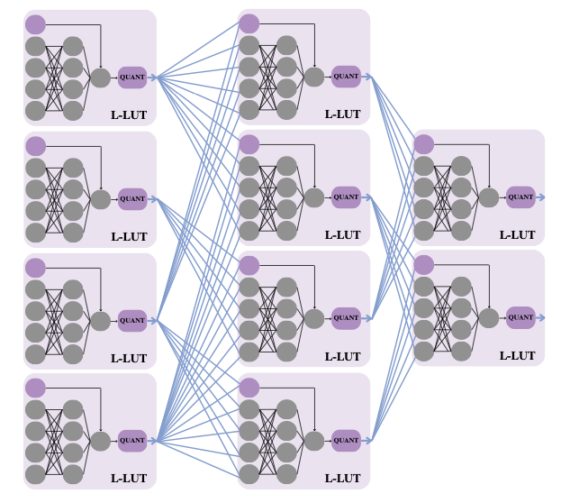
  lines in that function’s truth table. Since then, Marta and I have been exploring ways of parameterising that space to decouple the complexity of the function-classes implemented from the number of inputs. This gave rise to PolyLUT (parameterised as polynomials) and NeuraLUT (parameterised as small neural networks). Once we have learnt a function
  , all these methods enumerate the inputs of the function for the discrete space of quantised activations to produce the L-LUT. Olly’s work introduces `don’t cares’ into the picture: if a particular combination of inputs to the function is never, or rarely, seen in the training data, then the optimisation is allowed to treat the function as a don’t care at that point.

 , then I may as well be computing
  . In both cases, the fundamental issue becomes how to identify whether a value will be unused later in a computation. Intriguingly, this question is tightly related to the way a computation is performed: there are many ways of computing a given mathematical computation, and each one will have its own redundancies to exploit.
 and equivalences expressing clock and data gating within the same rewriting framework. A collection of these latter equivalences are shown in the table below from our paper.
 for its inputs
  and some learned weight vector
  and bias
  is typically a fixed nonlinear function such as a
  . The Xilinx team noted that if they restrict the length of the vector
  . In this way, we can tune a knob: turn down to
  for minimal expressivity but the smallest number of parameters to train, and recover LogicNets as a special case; turn up
 and
and  are the extracted “close” expressions.
 can just be replaced by
  , e.g.
  . But our original ARITH paper wasn’t able to consider special cases. What we really need for that is some kind of conditional rewrite rules, e.g.
  , where I am using math script to denote the value of a variable and teletype script to denote an expression.
 . Now let’s imagine introducing a new operator
  that takes two expressions, the second of which is interpreted as a Boolean. Let’s give
  . In this way we can ‘lift’ equivalences in a subdomain to equivalences across the whole domain, and use e-graphs without modification to reason about these equivalences. Taking the absolute value example from previously, we can write this equivalence as
  . These
 ![x \in [-1,1]](https://s0.wp.com/latex.php?latex=x+%5Cin+%5B-1%2C1%5D&bg=ffffff&fg=000000&s=0&c=20201002) , then a classical evaluation of
, then a classical evaluation of  would give me
 ![[-2,2]](https://s0.wp.com/latex.php?latex=%5B-2%2C2%5D&bg=ffffff&fg=000000&s=0&c=20201002) , due to the loss of information about the correlation between the left and right-hand sides of the subtraction operator. Once again, our e-graph setting comes to the rescue! Taking this example, a rewrite
, due to the loss of information about the correlation between the left and right-hand sides of the subtraction operator. Once again, our e-graph setting comes to the rescue! Taking this example, a rewrite  would likely fire, resulting in zero residing in the same e-class as
  . Since the interval associated with
  is
is ![[0,0]](https://s0.wp.com/latex.php?latex=%5B0%2C0%5D&bg=ffffff&fg=000000&s=0&c=20201002) , the same interval will automatically be associated with
, the same interval will automatically be associated with 

 of ‘hard’ samples I used to characterise the network varies in practice from the actual proportion