Precision Matters in Block Scales

This is the third post in a sequence relating to the geometry of block number formats as angle preservers. In my previous post, I argued that block number formats remain direction preservers even when their block scales are quantised all the way down to powers of two, as is common in some number representations like the MX concrete formats. The main result there was that exponent-only block scaling perturbs direction by at most about $20^\circ$ , and that $20^\circ$ is not that much in high dimensions. So we ended last time with the nice result that very coarse block-scale quantisation is relatively benign.

But that doesn’t mean power-of-two scaling is optimal. If we have a fixed budget of bits for representing block scales, how should we spend them? Specifically, should we spend them on exponent range, or on significand precision?

This post argues that the answer becomes much clearer once a high-precision tensor-wide scale is introduced, which is exactly the kind of two-level scaling used in NVIDIA’s NVFP4 format. In NVFP4, 4-bit E2M1 values are combined with an FP8 E4M3 scale for each 16-value micro-block and a second-level FP32 scale for the tensor.

With such a tensor-wide scale, the block scales are relieved of their duty to try to capture the global magnitude of the tensor. Instead, we can ask a more focused task of them: reconstruct the relative amplitudes of the blocks, so that the global direction of the represented vector is preserved.

Since drafting this post, Bardia Zadeh and I have also written Direction-Preserving Number Representations, which I blogged about separately. That paper studies the related question of what directions can be obtained when each coordinate of a vector is drawn from a finite scalar alphabet. This post is about block scales rather than scalar elements, but the same product-structured geometry reappears one level higher.

I will argue in this post that once we look at the problem that way, precision in the block scales starts to matter much more. This leads to a rough rule of thumb for the relationship between block scale formats and vector lengths.

What a tensor-wide scale changes

Suppose, as per my previous posts, that each block is represented as $\hat v_b = \beta_b^\star m_b$ , where $m_b$ is a chosen mantissa vector and $\beta_b^\star$ is the ideal real-valued block scale for that mantissa direction.

Now suppose that the final represented tensor has the form

$\tilde v = \gamma \bigoplus_{b=1}^K (\tilde \beta_b m_b)$

where

$\gamma$ is the high-precision tensor-wide scale,
$\tilde \beta_b$ is the low-precision per-block scale, and
$\bigoplus$ denotes direct sum (block concatenation).

Of course, the tensor-wide scale $\gamma$ has no effect on direction at all: it multiplies the whole tensor uniformly, so it only changes magnitude. That means the tensor-wide scale can be used to absorb the global length of the vector, leaving the block scales to encode relative block amplitudes.

In other words, once a tensor-wide scale is present, the block scales stop answering the question “how large is this tensor?” and instead answer the question “how do the blocks compare with one another?”

Exact scale-only cosine factor

Let $\hat v$ denote the ideal blockwise representation obtained using the real-valued scales $\beta_b^\star$ , and let $\tilde v$ denote the represented tensor after block-scale quantisation.

Write

$x_b = \frac{\tilde \beta_b}{\beta_b^\star}.$

Then the represented block is simply

$\tilde v_b = x_b \hat v_b.$

So scale quantisation does not change any chosen block direction, it only rescales the ideal projected blocks.

Define

$\alpha_b = \frac{|\hat v_b|^2}{\sum_j |\hat v_j|^2},$

so that $\alpha_b$ is the fraction of the ideal projected energy contained in block $b$ .

Then, exactly as in the previous post, we have

$\cos(\hat v,\tilde v) = \frac{\sum_b \alpha_b x_b}{\sqrt{\sum_b \alpha_b x_b^2}}.$

This says that directional distortion from block-scale quantisation depends only on how uneven the multiplicative scale errors $x_b$ are across blocks.

If all blocks were rescaled by the same factor, direction would be unchanged.

Two jobs for two different kinds of bits

A block-scale format does two things.

First, its exponent bits determine what range of relative block scales can be represented without clipping or underflow.

Second, its significand bits determine how accurately the in-range scales are represented.

So there are really two error sources:

tail loss, from blocks whose scales fall outside range;
in-range uneven rescaling, from finite precision within range.

The interesting question is how these trade off when the total number of scale bits is fixed.

A conservative scale-only view for fixed $K$

Suppose the tensor is divided into $K$ blocks.

If we want a format-level guarantee, a natural scale-only question is:

for a given number of blocks $K$ , how should a fixed budget of scale bits be split between exponent and significand so as to control the worst-case angular loss caused by scale quantisation?

I am deliberately saying “scale-only” here because this is not a claim about the globally optimal scalar alphabet (a problem Bardia and I cover in our preprint, linked to above), nor about the full problem of choosing the mantissa vectors. It is a conservative model of the additional angular error introduced after the block directions have already been chosen.

To make this concrete, let

$e$ be the number of exponent bits,
$p$ be the significand precision in bits, and
$k=e+p$ be the total scale-field width.

Now make one simplifying assumption: the mantissa vectors used in different blocks all have the same norm. Under that assumption, projected block energy is proportional to the square of the ideal block scale. This lets us reason directly in terms of the block scales themselves.

If the exponent field is too narrow, then very small relative block scales may underflow to zero after tensor-wide normalisation. In the worst case, one block survives at unit scale and the remaining $K-1$ blocks sit just below the lower threshold and are lost.

If the smallest representable normalised scale is $\tau_e$ , then the exponent-side cosine contribution is bounded by

$\displaystyle \cos(\hat v,z)\geq \frac{1}{\sqrt{1+(K-1)\tau_e^2}}.$

Here $z$ denotes the intermediate vector obtained by zeroing the blocks that fall below the representable scale threshold.

If, on the other hand, the surviving blocks remain in range but the scale precision is limited, then the remaining error comes from uneven in-range rescaling. Suppose the multiplicative scale errors for the surviving blocks satisfy

$\displaystyle \ell_p \leq x_b \leq u_p.$

Then the interval argument from the previous post gives

$\displaystyle \cos(z,\tilde v)\geq \frac{2\sqrt{\ell_p u_p}}{\ell_p+u_p}.$

In the common symmetric relative-error model, $\ell_p=1-u$ and $u_p=1+u$ , so this becomes

$\displaystyle \cos(z,\tilde v)\geq \sqrt{1-u^2}.$

Putting the clipping and in-range effects together gives the conservative scale-only bound

$\displaystyle \cos(\hat v,\tilde v)\geq \frac{2\sqrt{\ell_p u_p}}{\ell_p+u_p}\cdot \frac{1}{\sqrt{1+(K-1)\tau_e^2}}.$

In the symmetric relative-error model, this simplifies to

$\displaystyle \cos(\hat v,\tilde v)\geq \frac{\sqrt{1-u^2}}{\sqrt{1+(K-1)\tau_e^2}}.$

This is the key scale-only design inequality.

What this says about exponent bits

The first striking feature is that exponent bits only need to control the low-energy tail.

To make clipping negligible, it is enough to ensure that

$\displaystyle (K-1)\tau_e^2 \ll 1.$

Now the dynamic range of a floating-point-like scale grows extremely quickly with exponent width. A format-dependent way to write this is

$\displaystyle \tau_e \approx 2^{-c2^e},$

where $c$ is a positive constant depending on details such as exponent bias, reserved encodings, and whether subnormals are supported.

Substituting into the clipping condition gives

$\displaystyle (K-1)2^{-2c2^e}\ll 1.$

Solving this roughly gives

$\displaystyle e \gtrsim \log_2\log_2 K+O(1).$

The important point is the growth law. The number of exponent bits needed to control relative-tail clipping grows only like $\log\log K$ .

That is a very slow growth law: once $K$ is fixed, only a small number of exponent bits is needed before clipping becomes a second-order issue for direction.

What this says about significand bits

Once clipping is under control, the remaining scale error is dominated by in-range relative precision. That is the role of the significand.

In the symmetric relative-error model, the scale-only cosine contribution is

$\displaystyle \cos(z,\tilde v)\geq \sqrt{1-u^2}.$

Equivalently, the angular contribution is at most

$\displaystyle \arcsin(u).$

If a $p$ -bit significand gives a relative scale error of the form

$\displaystyle u\approx C_{\rm round}2^{-p},$

where $C_{\rm round}$ depends on the precise rounding convention, then asking the scale field alone to contribute at most an angle $\theta$ gives the rough condition

$\displaystyle C_{\rm round}2^{-p}\lesssim \sin\theta.$

Equivalently,

$\displaystyle p\gtrsim \log_2\left(\frac{C_{\rm round}}{\sin\theta}\right).$

So once the exponent field is “good enough”, every additional scale bit is more profitably spent on significand precision than on more dynamic range. This is the central conclusion of the scale-only model.

A simple rule of thumb

The previous discussion suggests the following design rule.

Use just enough exponent bits to make clipping of important blocks negligible. Spend the rest on significand precision.

For a tensor with $K$ blocks and a scale field of width $k$ , a rough rule of thumb is

$\displaystyle e^\star \approx \left\lceil \log_2\log_2 K \right\rceil + C_{\rm format},\qquad p^\star=k-e^\star.$

Here $C_{\rm format}$ is a small format-dependent additive correction – in a real format, it depends on details such as exponent bias, special encodings, and subnormal support. This is not meant as a precise optimum, only as a rough scale-only guide. But it makes the main point quite clearly:

exponent bits become sufficient very quickly; significand bits keep helping.

What this means for modern designs

This way of looking at the problem helps explain why a format that combines

a high-precision tensor-wide scale, and
a more precise block-scale format

looks like a very sensible design.

The tensor-wide scale deals with global magnitude. That leaves the block scales free to focus on preserving the relative block amplitudes that determine global direction.

This is exactly the tradeoff that makes NVFP4 interesting. Compared with exponent-only scaling, E4M3 block scales spend some representational power on non-power-of-two precision. The second-level FP32 tensor scale then compensates for the reduced range of the more precise E4M3 block-scale format.

There is also a useful connection with Bardia’s preprint. That paper studies the scalar alphabet inside a block, and finds that for 4-bit alphabets at the NVFP4 micro-block dimension $d=16$ , E2M1 is close to an independently optimized direction-preserving alphabet. This post studies a complementary question one level higher: once those micro-blocks have scales, how should the scale alphabet itself spend its bits?

So the two messages reinforce one another:

inside a micro-block, E2M1 is a surprisingly good product-structured scalar alphabet for direction preservation;
across micro-blocks, a tensor-wide scale makes the relative block-scale problem more important, so non-power-of-two block-scale precision becomes valuable.

From the perspective of directional reconstruction, that seems like a very good bargain.

Conclusion

The previous post showed that even exponent-only block scaling preserves direction surprisingly well.

This post goes a step further. Once a tensor-wide high-precision scale is available, the main question is no longer whether coarse block scaling is robust enough. Instead, we should ask whether the block scales are making the best possible use of their bits.

From the point of view of reconstructing global direction,

exponent bits protect against clipping of low-energy tail blocks;
significand bits improve the relative amplitudes of all the important in-range blocks.

Since exponent range grows very quickly with exponent width, only a modest number of exponent bits is needed before clipping becomes a secondary issue. After that, precision matters more.

This is a scale-only argument. It assumes the block directions have already been chosen, and studies the additional directional error caused by quantising the relative block amplitudes.

Proof sketch of the conservative scale-only bound

Readers not interested in the algebra can safely skip this section.

Assume equal mantissa norms across blocks, so that ideal projected block energy is proportional to the square of the ideal block scale.

Let $\hat v$ be the ideal blockwise projected vector after tensor-wide normalisation. We model low-precision block scales in two stages.

First, let $z$ be obtained from $\hat v$ by zeroing every block whose normalised scale falls below the smallest representable positive scale $\tau_e$ . In the worst case, one block survives at scale $1$ and the remaining $K-1$ blocks sit just below $\tau_e$ and are lost. The lost projected-energy fraction is then

$\displaystyle \eta=\frac{(K-1)\tau_e^2}{1+(K-1)\tau_e^2},$

$\displaystyle \cos(\hat v,z)=\sqrt{1-\eta}=\frac{1}{\sqrt{1+(K-1)\tau_e^2}}.$

Second, form the final represented vector $\tilde v$ by applying in-range rounding to the surviving block scales. If the surviving-block multiplicative errors satisfy

$\displaystyle \ell_p\leq x_b\leq u_p,$

then the interval bound from the previous post gives

$\displaystyle \cos(z,\tilde v)\geq \frac{2\sqrt{\ell_p u_p}}{\ell_p+u_p}.$

In the symmetric relative-error model, $\ell_p=1-u$ and $u_p=1+u$ , so this becomes

$\displaystyle \cos(z,\tilde v)\geq \sqrt{1-u^2}.$

Now write $\hat v=z+r$ , where $r$ is supported only on the clipped blocks. Since $\tilde v$ is supported only on the surviving blocks, we have $r\perp \tilde v$ , and hence

$\displaystyle \cos(\hat v,\tilde v)=\frac{\langle z,\tilde v\rangle}{|\hat v|_2|\tilde v|_2}=\frac{|z|_2}{|\hat v|_2}\frac{\langle z,\tilde v\rangle}{|z|_2|\tilde v|_2}=\cos(\hat v,z)\cos(z,\tilde v).$

Therefore

$\displaystyle \cos(\hat v,\tilde v)\geq \frac{2\sqrt{\ell_p u_p}}{\ell_p+u_p}\cdot \frac{1}{\sqrt{1+(K-1)\tau_e^2}}.$

In the symmetric relative-error model, this is

$\displaystyle \cos(\hat v,\tilde v)\geq \frac{\sqrt{1-u^2}}{\sqrt{1+(K-1)\tau_e^2}}.$

Directionality in Low Precision

In a couple of recent posts [1,2], I have been trying to reason through the geometric properties of block number formats. The basic idea is that when a group of numbers shares a scale factor, the small low-precision numbers inside the block are no longer meaningfully trying to approximate scalar magnitudes, as the scale has already taken care of much of the magnitude information. What remains is, to a significant extent, a question of direction.

This post is about a new preprint I have recently put out with Bardia Zadeh, “Direction-Preserving Number Representations”. The question we ask is “If a block scale has already taken care of magnitude, what should the scalar values inside the block look like if our aim is to preserve direction?”

That is not the usual question in computer arithmetic, and I can’t really find a historical precedent for this question in the usual places I would look (please let me know if you know others who have looked at this question from an arithmetic perspective!) We usually ask about absolute error, relative error, dynamic range, rounding behaviour, underflow, overflow, and so on. But in many modern machine learning settings, it is also natural to ask a more geometric question: how well do the values available inside a block cover the possible directions of a vector?

On the research methodology side, there is another aspect of this paper that is new for me personally. This is the first paper I have written where AI tools (namely GPT-5.4, GPT-5.5 and Aristotle) made a substantive contribution to the development of proof ideas, as well as to the Lean formalisation, which I am delighted we have open sourced. The AI tools definitely did not replace mathematical judgement or lead to a push button approach: the process still required many manual reformulations, checking, rewriting, and false starts. But it was a new and positive experience for me. In particular, the combination of exploratory AI assistance and Lean’s rock solid proof checking made for a very different style of research interaction from the one I am used to.

I will come back to Lean and AI below. First, let me describe the mathematical object we studied.

From scalar alphabets to directions

Suppose we have a finite scalar alphabet $A$ . For example, $A$ might be the set of real values represented by a 4-bit floating-point format, or by a 4-bit integer format.

If a block has dimension $n$ , then the unscaled vectors we can represent are the product set $A^n.$

But if the block also has an independent positive scale factor, then multiplying the whole vector by a positive scalar should not really change the information encoded by the low-precision elements. The scale can absorb that. What matters is the direction.

So the relevant object becomes

$P_n(A)=\left\{\frac{x}{|x|_2}:x\in A^n,\;x\ne 0\right\}.$

This is a finite set of points on the unit sphere. But these points can’t be placed arbitrarily on the sphere. The set has product structure, because each coordinate is chosen independently from the scalar alphabet.

The natural worst-case measure is the covering radius

$F_n(A)=\sup_{u\in S^{n-1}}\min_{c\in P_n(A)}\angle(u,c).$

This asks: given any true direction $u$ , how close is the nearest direction obtainable from the alphabet $A$ ? Smaller $F_n(A)$ is better.

This lens changes the problem of how to select the alphabet. Instead of asking “which scalar values approximate real numbers well?”, we ask: which scalar values, when used coordinatewise, cover directions well?

You can see the two-dimensional directionality coverage of the floating-point alphabet with two exponent bits, one mantissa bit and one sign bit (E2M1), illustrated below. Each intersection of grid lines corresponds to a 2-vector with elements drawn from this alphabet. We may then find where the line between the origin and that intersection meets a circle (marked as red points). Note the non-uniform spacing around the circle: some regions are better covered than others.

If you want to play with designing your own two-dimensional alphabet in a graphical user interface, you can get more intuition into this problem using this widget Bardia created: https://bardia01.github.io/directional_coverage_explorer/.

A Lean Interlude

As I mentioned above, I’m super pleased that we’ve open-sourced formalisations of all our theorems and definitions in Lean. The formalisation is organised so that the top-level declarations correspond closely to the paper.

The key definitions look like this:

abbrev Aq (q : Nat) : Set (Finset Real) :=
  {A : Finset Real | A.card = q}

abbrev P (n : Nat) (A : Finset Real) :
  Finset (OptimalAlphabets.SpherePoint n) :=
  OptimalAlphabets.AsymmetricProduct.asymProdSphericalCode n A

abbrev F (n : Nat) (A : Finset Real) : Real :=
  OptimalAlphabets.AsymmetricProduct.F_asym n A

abbrev rhoSph (n m : Nat) : Real :=
  OptimalAlphabets.rho_sph n m

Here Aq q is the class of scalar alphabets with $q$ elements. The definition P n A is the finite spherical code obtained by normalising nonzero elements of $A^n$ . The quantity F n A is the product-code covering objective $F_n(A)$ . The definition rhoSph n m is the optimal covering radius of an unconstrained spherical code with $m$ points.

I’m giving these Lean definitions now so we can roughly follow along in Lean as we go for the rest of this blog post.

Product Codes versus Spherical Codes

It seems natural, almost obvious, that a product code should give worse directional coverage than a vector code chosen specifically to optimise directional coverage. Of course, the latter may not be practical, as the decoding process may be significant, but it still forms a useful baseline comparison point. Our first theoretical contribution is to quantify the gap between these two code classes.

Notice that the product structure induces a very severe geometric constraint. Even if $A$ has $q$ values, so that $A^n$ has up to $q^n$ raw vectors, those vectors are not arbitrary. They arise from independent coordinate choices from the same scalar alphabet. Meanwhile, a spherical code with $q^n$ points is free to place those points anywhere on the sphere.

The harmonic witness

A central construction in the paper is a direction that is hard for product codes to cover. Let

$H_n=\sum_{i=1}^{n}\frac{1}{i}$

be the $n$ th harmonic number, and define the unit vector

$u^{(n)}=\left(\frac{1}{\sqrt{H_n}},\frac{1}{\sqrt{2H_n}},\ldots,\frac{1}{\sqrt{nH_n}}\right).$

The entries of this vector decay slowly, making the vector awkward for a finite scalar alphabet. The resulting theorem gives a lower bound on the worst-case angular error. If $m(A)$ is the smaller of the number of positive and negative nonzero values in $A$ , then

$F_n(A)\ge \arccos\left(\min\left\{1,\;2\sqrt{\frac{m(A)}{H_n}}\right\}\right).$

The Lean statement is compact enough to include directly:

theorem theorem2_sign_count_bound {n : Nat} (hn : 2 <= n)
    (A : Finset Real) :
  Real.arccos
    (min 1 (2 * Real.sqrt (mSign A : Real) / Real.sqrt (H n))) <=
  F n A

The notation mSign A is the Lean name for $m(A)$ , the smaller nonzero sign count. The theorem is written as a lower bound on F n A, just as in the paper.

Since $H_n$ grows like $\log n$ , this bound tends towards $\pi/2$ for any fixed alphabet. In plain language: in sufficiently high dimension, every fixed scalar alphabet has some direction that it represents very badly.

This is a worst-case theorem. We’re not claiming that real neural network tensors look like the harmonic witness. What the theorem tells us is that if the metric is worst-case angular coverage of the entire sphere, product-structured scalar alphabets have an inherent limitation.

So What about Spherical Codes?

A product code built from a $q$ -element alphabet has at most $q^n$ raw codewords before normalisation. The fair unconstrained comparison is therefore a spherical code with $q^n$ points.

The paper proves that, for any fixed $q$ , sufficiently high-dimensional spherical codes beat every $q$ -element product code in worst-case angular covering radius.

Here is the Lean statement:

theorem theorem4_asymptotic_strict_separation_fixed_alphabet_size
    {q : Nat} (hq : 2 <= q) :
  ∃ N : Nat, 2 <= N ∧
    forall n, N <= n ->
      forall A : Finset Real, A ∈ Aq q ->
        rhoSph n (q ^ n) < F n A

Read from right to left, this says: take any scalar alphabet $A$ with $q$ elements. In all sufficiently large dimensions $n$ , the best unconstrained spherical code with $q^n$ points has strictly smaller covering radius than the product-code direction set induced by $A$ .

What about Floating and Fixed Point?

The next question we answer is more practical. Within the product-code world, are the usual scalar alphabets the best ones?

The paper studies standard floating-point, fixed-point, and two’s complement alphabets. The answer is that these conventional choices are asymptotically suboptimal for the worst-case directional metric.

Because the worst-case angle for any product code tends towards $90^\circ$ in high dimension (see above), it is more informative when comparing product codes to look at a normalised quantity such as:

$\sqrt{H_n}\cos F_n(A).$

Very roughly, this measures how slowly the worst-case angle approaches $90^\circ$ . Larger is better.

The Lean statement packages the relevant comparison as a liminf/limsup chain:

theorem theorem5_liminf_limsup_chain {b : Nat} (hb : 3 <= b) :
  arbConst b <=
      Filter.liminf (fun n : Nat => normBestAlpha n (2 ^ b)) atTop ∧
  fpConst b < arbConst b ∧
  Filter.limsup (fun n : Nat => normBestFpCos n b) atTop <= fpConst b

This is a theorem about $b$ -bit alphabets. The quantity normBestAlpha n (2 ^ b) is the best normalised performance obtainable by an arbitrary $2^b$ -element scalar alphabet. The quantity normBestFpCos n b is the corresponding floating-point quantity, optimised over valid splits of exponent and mantissa bits. The constants arbConst b and fpConst b are the two asymptotic constants being compared.

The middle inequality fpConst b < arbConst b is the key point. For $b\ge 3$ , arbitrary scalar alphabets can do strictly better than the floating-point family in this asymptotic directional metric.

For four bits, the paper obtains a concrete constant-factor separation of at least $\sqrt{7/3}\approx 1.528.$

So if the design objective is “choose scalar levels whose product code covers directions well”, there are better alphabets than the standard ones, at least in this worst-case asymptotic sense.

AI and Lean

It feels worth saying a little more about the process followed to reach the proofs of these theorems. This paper is the first time I have had a genuinely substantive AI contribution to the development of proof ideas, not just text polishing and review. AI was useful both in the Lean formalisation and in exploring how some of the mathematical arguments might be structured.

The AI tools we used needed lots of iteration, but the workflow was unexpectedly productive. GPT-5.4 and 5.5 and Aristotle from Harmonic could suggest possible routes, propose intermediate lemmas, help with translation between informal mathematics and Lean statements, and generate candidate proof fragments.

This combination was new for me. I am used to mathematical collaboration involving conversations with people, paper sketches, whiteboards, and eventually LaTeX. Here there was another kind of interaction: a fast, imperfect, but useful assistant for exploring the proof space, coupled with Lean as a formal system that refused to accept anything vague.

Mathematical judgement still matters, in what we wanted to prove as well as what counts as an informative proof. But I came away from the experience more positive about the role these tools can play in research, especially when paired with formal verification rather than used as a substitute for it.

The Experimental Side: Exploring 4-bit Alphabets

The theory says that better scalar alphabets should exist. The experiments in the paper ask what they look like. For four-bit alphabets, we impose sign symmetry and include zero. Since multiplying all scalar levels by a common positive factor does not change the represented directions, we normalise the smallest positive value to one.

For block dimension $d=16$ (as used in NVIDIA NVFP4), the optimised positive levels found in the paper are approximately

$1,\;2.12,\;3.40,\;5.04,\;7.25,\;10.5,\;13.2.$

The optimised alphabet is best across the tested dimensions. But what I find most interesting is how close E2M1 is to the optimum, especially compared with integer/fixed-point and pure powers-of-two formats.

E2M1 is the four-bit format used in NVFP4. The results suggest a geometric explanation for why it works well in block-scaled machine learning settings. The key point is that, for this bit-width and block size, the E2M1 levels lie surprisingly close to the levels obtained by directly optimising the product-code directional covering problem.

Conclusion

The main message is that the geometric lens provides value when considering how to design low-precision number formats for machine learning. Once a block scale is present, the scalar values inside the block are not merely approximating real numbers independently. Together, they are choosing a direction. The scalar alphabet therefore determines a product-structured spherical code.

There are three consequences I find useful.

First, product structure has unavoidable limitations. A coordinatewise scalar alphabet cannot cover directions as well as an unconstrained spherical code with the same number of raw codewords.

Second, standard scalar formats are not forced by the geometry. Floating-point, fixed-point, and two’s complement are natural formats for many reasons, but the directional covering objective points to other possibilities.

Third, E2M1 comes out looking very good. The optimised alphabet is better in the sampled worst-case metric, but E2M1 is close enough that its empirical success in block-scaled low-precision settings has a clean geometric explanation.

The Lean formalisation matters because it pins down the definitions, checks the asymptotic comparisons, verifies the separation from standard formats, and formalises the scale-search theorem used in the experiments.

The AI aspect matters to me for a different reason. It changed the way this paper was developed. The experience was not one of handing mathematics over to a machine, but of using AI as part of a proof-development workflow. For me, that was new, and it was positive.

So perhaps a promising design question for future low-precision formats should be phrased less like the traditional “Which scalar values approximate real numbers best?” and more like “Which scalar values, when used coordinatewise inside a block, represent directions best?” That seems like a useful question in the world of block-scaled arithmetic.

AI in Education

In the UK, the Parliamentary Select Committee on Education is currently holding an inquiry into “The use of Artificial Intelligence and EdTech in Education”. I am reproducing my submission to this inquiry below, in case it is of value to others. The text can also be found – alongside all other submissions made – at the official parliamentary website.

AIE0024 Download

Block Number Formats are (Still!) Direction Preservers

In my previous post, I argued that block number formats can be understood geometrically as direction preservers. That argument relied on an idealization: once a block direction had been chosen, its scale could be set optimally as an arbitrary real number.

Real hardware formats do not usually work that way. In many practical schemes, block scales are quantized very coarsely, sometimes all the way down to powers of two. In particular, in the MX specification, all the concrete compliant formats use E8M0 scaling.

So does the directional picture I painted in my last post survive this brutal scaling? Here I will argue, in the first of what I hope will be a short sequence of follow-up blog posts, that it does.

From ideal block scales to quantized block scales

Recall the setup from the earlier post. A vector is partitioned into blocks, $v = (v_1,\dots,v_B)$ , and each block is approximated as $\hat v_b = \beta_b m_b$ , where $m_b$ is a low-precision mantissa vector and $\beta_b$ is a scalar block scale.

In the earlier post, I assumed that $\beta_b$ was an arbitrary real value, chosen optimally in the least-squares sense. That gave the ideal blockwise representation $\hat v$ .

Now let us keep the same mantissa vectors $m_b$ , but suppose that the scale factors themselves must be quantized. Write the implemented scale as $\tilde \beta_b$ , so that the represented block becomes $\tilde v_b = \tilde \beta_b m_b$ .

It is convenient to define the multiplicative scale error $x_b = \frac{\tilde \beta_b}{\beta_b}$ . Then $\tilde v_b = x_b \hat v_b$ .

Note that, of course, quantizing the block scale does not change the chosen direction of a block at all; it only changes its length. So the only directional distortion comes from the relative rescaling of different blocks.

An exact cosine formula

Let $\alpha_b = \frac{\|\hat v_b\|^2}{\sum_j \|\hat v_j\|^2}$ , so that $\alpha_b$ is the fraction of the ideal projected vector’s energy contained in block $b$ .

Then it can be shown that $\cos(\hat v,\tilde v) = \frac{\sum_b \alpha_b x_b}{\sqrt{\sum_b \alpha_b x_b^2}}$ (the proof is included at the end of this post).

So the effect of scale quantization on direction depends only on how uneven the factors $x_b$ are across blocks. If all blocks were rescaled by the same factor, direction would be unchanged.

Exponent-only power-of-two scaling

Now consider the coarsest plausible case: each block scale is rounded to the nearest power of two. Then each multiplicative error satisfies $x_b \in [2^{-1/2},\,2^{1/2}]$ .

So, from our exact cosine formula, we are interested in how small $\frac{\sum_b \alpha_b x_b}{\sqrt{\sum_b \alpha_b x_b^2}}$ can be, when all the $x_b$ lie in the interval $[2^{-1/2},\,2^{1/2}]$ .

A simple inequality shows that the answer depends only on the two extreme values of the interval. If all the block rescaling factors lie in $[\ell,u]$ , then

$\frac{\sum_b \alpha_b x_b}{\sqrt{\sum_b \alpha_b x_b^2}}\ge \frac{2\sqrt{\ell u}}{\ell+u}$ (proof at the end of this blog post).

In the power-of-two case we have $\ell=2^{-1/2}$ , $u=2^{1/2}$ , so $\ell u=1$ , and therefore

$\cos(\hat v,\tilde v)\ge \frac{2}{2^{-1/2}+2^{1/2}} = \frac{2\sqrt2}{3}\approx 0.943$ .

Equivalently, $\angle(\hat v,\tilde v)\le 20^\circ$ .

So even if every block scale is rounded to the nearest power of two, the resulting vector remains within about $20^\circ$ of the ideally scaled one.

That is the main result of this post.

One striking feature of the bound is that it does not depend on the dimension of the vector. The reason is that the worst case is already attained by a two-group energy split: some blocks rounded up, others rounded down. Once those two groups exist, adding more blocks or more dimensions does not make the bound worse, as is apparent from the proof below.

20 degrees is less than it sounds

Our everyday intuition may tell us that this angle is not huge, but it’s not that small either. In a sense, that’s true. But angles behave very differently in high-dimensional spaces. In high dimension, most random vectors are almost orthogonal to one another: their angle is close to $90^\circ$ , so a guarantee that an approximation remains within $20^\circ$ of the original vector is much stronger than it would sound in two or three dimensions.

Beyond power-of-two

We’ve analysed power-of-two scaling here for two reasons: because it’s in a sense the crudest possible floating-point rounding, and because it’s commonly used in real hardware designs.

That does not mean it’s optimal. But it does raise two further questions. Firstly, we’ve assumed here that the exponent range is sufficiently wide – what if it’s not? Secondly – and relatedly – how much better can this angular bound get by spending some of the scale bits on greater precision?

My view is that the answer becomes clearer once a tensor-wide high-precision scale is introduced, something NVIDIA has recently done. In that setting, the block scales get relieved of their additional duty to capture global magnitude. This will be the subject of the next post on the topic!

Proofs

Readers not interested in the algebra can safely skip this section.

Cosine formula

Recall that $\tilde v_b = x_b \hat v_b$ for each block $b$ .

Then, because the blocks occupy disjoint coordinates, $\langle \hat v,\tilde v\rangle = \sum_b \langle \hat v_b,\tilde v_b\rangle = \sum_b x_b \|\hat v_b\|^2$ .

Therefore $\cos(\hat v,\tilde v) = \frac{\langle \hat v,\tilde v\rangle}{\|\hat v\|\,\|\tilde v\|} = \frac{\sum_b x_b \|\hat v_b\|^2}{\sqrt{\sum_b \|\hat v_b\|^2}\sqrt{\sum_b x_b^2 \|\hat v_b\|^2}}$ .

Now, as per the main blog post, define $\alpha_b = \frac{\|\hat v_b\|^2}{\sum_j \|\hat v_j\|^2}$ .

Writing $S=\sum_j \|\hat v_j\|^2$ , so that $\|\hat v_b\|^2=\alpha_b S$ , the numerator becomes $S\sum_b \alpha_b x_b$ and the denominator becomes $S\sqrt{\sum_b \alpha_b x_b^2}$ , giving

$\cos(\hat v,\tilde v)=\frac{\sum_b \alpha_b x_b}{\sqrt{\sum_b \alpha_b x_b^2}}$ .

$\square$

20 degree bound

Assume that all the multiplicative error factors lie in an interval $x_b \in [\ell,u]$ with $u > \ell > 0$ .

Let $\mu := \sum_b \alpha_b x_b,\qquad q := \sum_b \alpha_b x_b^2$ .

Then the cosine is just $\mu/\sqrt q$ . Since each $x_b\in[\ell,u]$ , we have

$(x_b-\ell)(x_b-u)\le 0$ .

Expanding this gives

$x_b^2 \le (\ell+u)x_b - \ell u$ .

Multiplying by $\alpha_b$ and summing over $b$ gives

$q \le (\ell+u)\mu - \ell u$ .

Therefore $\frac{\mu^2}{q}\ge \frac{\mu^2}{(\ell+u)\mu-\ell u}$ .

Now the weighted mean $\mu$ also lies in the interval $[\ell,u]$ , so it remains to minimize

$\frac{\mu^2}{(\ell+u)\mu-\ell u}$ over $\mu\in[\ell,u]$ .

Differentiating shows that the minimum occurs at $\mu=\frac{2\ell u}{\ell+u}$ , the harmonic mean of $\ell$ and $u$ .

Substituting this value gives

$\frac{\mu^2}{q}\ge \frac{4\ell u}{(\ell +u)^2}$ ,

and therefore

$\frac{\mu}{\sqrt q}\ge \frac{2\sqrt{\ell u}}{\ell +u}$ .

So we have proved that

$\frac{\sum_b \alpha_b x_b}{\sqrt{\sum_b \alpha_b x_b^2}}\ge \frac{2\sqrt{\ell u}}{\ell+u}$ .

Finally, in the power-of-two case we have

$\ell=2^{-1/2}$ and $u=2^{1/2}$ , so $\ell u=1$ , and hence

$\cos(\hat v,\tilde v)\ge \frac{2}{2^{-1/2}+2^{1/2}} = \frac{2\sqrt2}{3}$ .

Numerically,

$\frac{2\sqrt2}{3}\approx 0.943$ ,

$\angle(\hat v,\tilde v)\le \arccos\left(\frac{2\sqrt2}{3}\right) < 20^\circ$ .

$\square$

Block Number Formats are Direction Preservers

I’ve recently returned from the SIAM PP 2026 conference and as always, conferences help provide time for research reflection. One thing I’ve been reflecting on during my journey back is the various explanations people give for why the machine learning world is so keen on block number formats (MX, NVFP, etc.) – see my earlier blog post on MX if you need a primer. Many hardware engineers tend to answer that they lead to efficient storage, or efficient arithmetic, or improved data transfer bandwidth, which are all true. But I think there’s another complementary answer that’s less well discussed (if indeed it is discussed at all). I hope this blog post might help stimulate some discussion of this complementary take.

On the numerical side, at first glance it might seem surprising that despite these formats representing numbers with very limited precision, large neural networks often tolerate them remarkably well, with little loss in accuracy. In my experience, most explanations focus on dynamic range, quantization noise, the inherent noise robustness of neural networks, or calibration techniques. But I suspect there is also a simple geometric way to think about what these formats are doing: Block number formats help preserve vector direction. And for many machine learning computations, preserving direction matters far more than preserving exact numerical values.

Block formats inherently represent direction and magnitude

Consider a vector $v$ whose coordinates are partitioned into blocks $v = (v_1, v_2, \dots, v_B)$ .

In a block format, each block is represented using a shared scale and low-precision mantissas. For ease of discussion, we’ll consider the simplest case here, where scales are allowed to be arbitrary real-valued. In general, they may be much more restricted, e.g. powers of two.

Each block is approximated as $\hat v_b = \beta_b m_b$

where

$m_b$ is a vector of low-precision mantissas, and

$\beta_b$ is a scalar shared scaling factor.

In other words, each block can be thought of as a direction (encoded by the mantissas) multiplied by a magnitude (the shared scale). Strictly speaking, the mantissa vectors $m_b$ need not be normalized, and in many formats their entries may have quite different magnitudes (for example in integer mantissa formats such as MXINT). However this does not change the geometry. The representation $\hat{v}_b = \beta_b m_b$ is invariant to rescaling of $m_b$ : multiplying $m_b$ by any constant simply rescales $\beta_b$ by the inverse factor. What matters for the approximation is therefore only the direction of $m_b$ , i.e. the one-dimensional subspace it spans.

Often we don’t think of it like this, but broadly speaking this is what has happened: block scaling allows us to decouple magnitude and direction representation. This resembles the familiar decomposition $v = \|v\|\frac{v}{\|v\|}$ of a vector into its magnitude and direction, but applied locally within blocks.

If the mantissa vector $m_b$ points roughly in the same direction as the original block $v_b$ , then scaling it appropriately produces a good approximation of that block.

OK, but does preserving directions block by block actually preserve the direction of the whole vector? It turns out that the answer is yes.

Direction Preservation

Let us make the reasonable assumption that the scale of each block $\beta_b$ is not chosen arbitrarily, but rather is the best possible scale for that block in the least squares sense, for whatever mantissa vector we choose, i.e. $\beta_b = \arg\min_{\beta} \|v_b - \beta m_b\|^2$ . Then $\hat v_b$ is the orthogonal projection of $v_b$ onto the line spanned by $m_b$ .

So to what extent do the approximate and the original block vector point in the same direction? We can measure the block cosine similarities of the blocks as: $\rho_b = \frac{\langle v_b,\hat v_b\rangle}{\|v_b\|\|\hat v_b\|}$ .

Equally, we can measure the the cosine similarity of the full vectors (the concatenation of the original blocks versus the concatenation of the approximated blocks): $\rho = \frac{\langle v,\hat v\rangle}{\|v\|\|\hat v\|}$ .

My aim here is to explain why small error in direction at block level leads to small error at vector level.

First, let’s define $w_b = \frac{\|v_b\|^2}{\|v\|^2}$ , which we can think of as the fraction of the vector’s energy contained in block $b$ ; these add to 1 over the whole vector. Now we can state the result:

Theorem (Block Cosines)

Under the blockwise least-squares scaling, $\rho = \sqrt{\sum_{b=1}^{B} w_b \rho_b^2 }$ .

For proof, see end of post.

In simple terms, this theorem states that the cosine similarity of the whole vector is the energy-weighted RMS of the block cosine similarities.

What are the implications?

The weights $w_b$ represent how much of the vector’s energy lies in each block. Blocks that contain very little energy contribute very little to the final direction. The important consequence is that direction errors do not accumulate catastrophically across blocks. Instead, the overall directional error simply depends on a weighted average of the block direction errors. In other words, if block number formats preserve the directions of individual blocks, they automatically preserve the direction of the entire vector.

Many core operations in machine learning depend heavily on vector direction. Notably, during training, stochastic gradient descent updates are already in the form of magnitude (learning rate) + direction. We already have a knob controlling magnitude (the learning rate); what matters is that the direction is preserved. In attention mechanisms and embedding, directional similarity measures are very important. Even for the humble dot product, the workhorse of inference, preservation of direction means that small perturbations in input give rise to only small perturbations in output, so the dot product behaves robustly.

Conclusion

Block floating-point and similar formats like block mini-float, MX, NVFP, are usually explained in terms of dynamic range and quantization noise. But geometrically, I like the perspective that they do something simpler: they approximate each block of a vector as direction × magnitude.

And as long as the block directions are preserved reasonably well, the direction of the whole vector is preserved too.

I think this is a useful intuition as to why very low-precision formats can work so well in modern machine learning systems. Block number formats are, in a very real sense, direction preservers. From this perspective, such low-precision block formats succeed not because they represent individual numbers accurately, but because they preserve the geometry of vectors.

Lots of extensions of this kind of analysis are of course possible. To name just a few:

We’ve focused on vectors, but tensor-level scaling may have interesting interplay with batching during training, for example
We made the simplifying assumption that scaling factors were real valued, but these can be restricted, most significantly to powers of two, and the analysis would need to be modified to incorporate that change.
We’ve not discussed mantissas at all, lots more of interest could be said here.
Potentially this approach could help provide some guidance to the empirical sizing of blocks in a block representation.

If anyone would like to work with me on this topic, do let me know your ideas.

Proof of the theorem

Readers not interested in the algebra can safely skip this section.

For each block $b$ , the approximation $\hat v_b = \beta_b m_b$ with $\beta_b$ chosen by least squares is the orthogonal projection of $v_b$ onto the line spanned by $m_b$ .

So we can write $v_b = \hat v_b + r_b$ where $r_b$ is orthogonal to $\hat v_b$ .

Taking the inner product with $\hat v_b$ gives $\langle v_b,\hat v_b\rangle = \|\hat v_b\|^2$ .

Now sum over blocks. Because the blocks correspond to disjoint coordinates,

$\langle v,\hat v\rangle = \sum_b \langle v_b,\hat v_b\rangle = \sum_b \|\hat v_b\|^2 = \|\hat v\|^2$ .

Therefore

$\rho = \frac{\langle v,\hat v\rangle}{\|v\|\|\hat v\|} = \frac{\|\hat v\|}{\|v\|}$ .

Recall $\rho_b = \frac{\langle v_b,\hat v_b\rangle}{\|v_b\|\|\hat v_b\|}$ .

Using $\langle v_b,\hat v_b\rangle=\|\hat v_b\|^2$ , we obtain

$\rho_b = \frac{\|\hat v_b\|}{\|v_b\|}$ .

Hence

$\|\hat v_b\|^2 = \rho_b^2 \|v_b\|^2$ .

Summing over blocks gives

$\|\hat v\|^2 = \sum_b \|\hat v_b\|^2 = \sum_b \rho_b^2 \|v_b\|^2$ .

Dividing by $\|v\|^2$ , and writing

$w_b = \frac{\|v_b\|^2}{\|v\|^2}$ ,

gives

$\frac{\|\hat v\|^2}{\|v\|^2} = \sum_b w_b \rho_b^2$ .

Since $\rho = \|\hat v\|/\|v\|$ , we obtain

$\rho = \sqrt{\sum_b w_b \rho_b^2 }$ .

$\square$

California / FPGA 2026

This month I took a trip to California for the FPGA 2026 conference, together with my two new PhD students Ben Zhang and Bardia Zadeh, which I combined with a number of visits in the San Francisco Bay Area in the days preceding the conference. This post provides a brief summary of my visit.

First up on our travels was dinner with Rocco Salvia. Rocco was my Research Assistant – we worked together some years ago on automating the analysis of average-case numerical behaviour of reduced-precision floating-point computation. He is now working for Zoox, the robotaxi company owned by Amazon where his first-rate engineering skills are being put to good use!

The following day we went to visit Max Willsey at UC Berkeley and his PhD student Russel Arbore. Max and I (together with others) organised a Dagstuhl workshop on e-graphs recently, and we went to pick up the research conversations we left behind a month ago in Germany and spend some good quality whiteboard time together. Russel and Max are working on some really exciting problems in program analysis.

That afternoon, we had the chance to catch up with my old friend and colleague Satnam Singh, now working for the startup harmonic.fun. Harmonic is a really exciting company, combining modern AI tools with Lean-based formal theorem proving. Expect great things here.

George, Satnam, Bardia and Ben, enjoying coffee near the Harmonic office.

The following morning, we went to visit AMD, with whom I have longstanding collaborations. Amongst others, we met my two former PhD students Sam Bayliss and Erwei Wang there, and discussed our ongoing work on e-graphs and on efficient machine learning, as well as finding out the latest work in Sam’s team at AMD including their release of Triton-XDNA.

That afternoon we visited NVIDIA’s stunning HQ to meet with Rajarshi Roy and Atefeh Sohrabizadeh. I know both of them through the EPSRC International Centre-to-Centre grant I led: Rajarshi was introduced to me by Bryan Catanzaro as the author of some really interesting work on reinforcement learning for computer arithmetic design, and spoke at our EPSRC project’s annual workshop. Atefeh was a PhD student affiliated with the Centre (advised by Jason Cong, UCLA) and spent some time visiting my research group. We heard about the recent NVIDIA work on AI models to aid software engineering and of combined speech and language.

Rajarshi, Ben, Bardia, George and Atefeh at NVIDIA

It has long been a tradition that Peter Cheung, when in the Bay Area, organises a get-together of alumni of the Circuits and Systems Group (formerly Information Engineering group, when Bob Spence was Head of Group). This time was no exception – we met up with many of our department’s former students, and some came to a great dinner too. It’s always a delight to hear about the activity of our alumni, spread across the tech companies in the Bay Area.

After a flying visit to my former PhD student’s family, we then made it down to Monterey for FPGA 2026. Regular readers of this blog will know that I’ve been attending FPGA for more than 20 years, have been Program Chair, General Chair, Finance Chair and am now Steering Committee member of the conference. So it always feels a little like “coming home”. I also love Monterey – despite the touristy bits – and am a fan of Steinbeck‘s writing in which he immortalised Monterey with some of the best opening lines ever (of Cannery Row): “Cannery Row in Monterey in California is a poem, a stink, a grating noise, a quality of light, a habit, a nostalgia, a dream.”

This year, the general chair of FPGA 2026 was Jing Li, and the great programme was put together by Grace Zgheib.

My favourite paper at FPGA this year also won the best paper prize. Duc Hoang and colleagues identified that Kolmogorov-Arnold Networks are a natural fit to the LUT-based neural networks my group pioneered e.g. [1,2]. They form a really interesting design point, overcoming the exponential scaling of area with the product of precision and neuron fanin present in both my SOTA work with Marta Andronic and earlier work like Xilinx LogicNets, to produce a design that scales exponentially only in the precision. I very much enjoyed reading this paper and seeing it presented, and I think it opens up new areas of future work in this area.

Duc Hoang and his coauthor Aarush Gupta, receiving the best paper award from Grace and Jing

I also particularly enjoyed the work of Shun Katsumi, Emmet Murphy and Lana Josipović (ETH Zurich) on eager execution in elastic circuits. I previously collaborated with Lana on elastic circuits, and it’s great to see the latest work in this area and the use of formal verification tools to prove correctness of performance enhancements. I had a very nice discussion with Lana about possible ways to take this work further.

Rouzbeh Pirayadi, Ayatallah Elakhras, Mirjana Stojilović and Paolo Ienne (EPFL) had a really interesting paper on avoiding the overhead of load-store queues in dynamic high-level synthesis. (This paper was also the runner-up best paper).

From my own institution, Oliver Cosgrove, Ally Donaldson and John Wickerson had a great paper on fuzzing FPGA place and route tools, which has led a vendor to fix a bug they uncovered through their tool.

There were many other good papers, but just to mention a couple that I found particularly aligned to my own interests: EdgeSort on the design of line-rate streaming sorters and HACE on extracting CDFGs from RTL were both really interesting to hear presented.

It was great to be reunited with so many international colleagues and to provide my new students Bardia and Ben with the chance to begin their journey of integration into this welcoming community.

Me, John, Bardia, Oliver and Ben after the end of the final conference session

FCCM 2025

I’ve recently returned from the IEEE International Symposium on Field-Programmable Custom Computing Machines (known as FCCM). I used to attend FCCM regularly in the early 2000s, and while I have continued to publish there, I have not attended myself for some years. I tried a couple of years ago, but ended up isolated with COVID in Los Angeles. In contrast, I am pleased to report that the conference is in good health!

The conference kicked off on the the evening of the 4th May, with a panel discussion on the topic of “The Future of FCCMs Beyond Moore’s Law”, of which I was invited be be part, alongside industrial colleagues Chris Lavin and Madhura Purnaprajna from AMD, Martin Langhammer from Altera, and Mark Shand from Waymo. Many companies have tried and failed to produce lasting post-Moore alternatives to the FPGA and the microprocessor over the decades I’ve been in the field and some of these ideas and architectures (less commonly, associated compiler flows / design tools) have been very good. But, as Keynes said, “markets can remain irrational longer than you can remain solvent”. So instead of focusing on commercial realities, I tried to steer the panel discussion towards the genuinely fantastic opportunities our academic field has for a future in which power, performance and area innovation changes become a matter of intellectual advances in architecture and compiler technology rather than riding the wave of technology miniaturisation (itself, of course, the product of great advances by others).

The evening panel, as imagined by AI. I’m 2nd to left. The AI tool was clearly unaware of Martin’s height difference!

The following day, the conference proper kicked off. Some highlights for me from other authors included the following papers aligned with my general interests:

AutoNTT: Automatic Architecture Design and Exploration for Number Theoretic Transform Acceleration on FPGAs from Simon Fraser University, presented by Zhenman Fang.
RealProbe: An Automated and Lightweight Performance Profiler for In-FPGA Execution of High-Level Synthesis Designs from Georgia Tech, presented by Jiho Kim from Callie Hao‘s group.
High Throughput Matrix Transposition on HBM-Enabled FPGAs from the University of Southern California (Viktor Prasanna‘s group).
ITERA-LLM: Boosting Sub-8-Bit Large Language Model Inference Through Iterative Tensor Decomposition from my colleague Christos Bouganis‘ group at Imperial College, presented by Keran Zheng.
Guaranteed Yet Hard to Find: Uncovering FPGA Routing Convergence Paradox from Mirjana Stojilovic‘s group at EPFL – and winner of this year’s best paper prize!

In addition, my own group had two full papers at FCCM this year:

Banked Memories for Soft SIMT Processors, joint work between Martin Langhammer (Altera) and me, where Martin has been able to augment his ultra-high-frequency soft-processor with various useful memory structures. This is probably the last paper of Martin’s PhD – he’s done great work in both developing a super-efficient soft-processor and in forcing the FPGA community to recognise that some published clock frequency results are really quite poor and that people should spend a lot longer thinking about the physical aspects of their designs if they want to get high performance.
NeuraLUT-Assemble: Hardware-aware Assembling of Sub-Neural Networks for Efficient LUT Inference, joint work between my PhD student Marta Andronic and me. I think this is a landmark paper in terms of the results that Marta has been able to achieve. Compared to her earlier NeuraLUT work which I’ve blogged on previously, she has added a way to break down large LUTs into trees of smaller LUTs, and a hardware-aware way to learn sparsity patterns that work best, localising nonlinear interactions in these neural networks to within lookup tables. The impact of these changes on the area and delay of her designs is truly impressive.

Martin explaining efficient
memory structures for soft processors

Overall, it was well worth attending. Next year, Callie will be hosting FCCM in Atlanta.

FPGA & HPCA 2025

I recently returned from two back-to-back conferences, FPGA 2025 in Monterey, California and HPCA 2025 in Las Vegas, Nevada. In this blog post, I will summarise some of the things I found most interesting at these conferences.

Before I even got to the first conference, I was delighted to have the chance to meet in San Francisco with Cole Harry, who runs the new Imperial Global USA. They have an exciting plan of work to develop links between Imperial and academics, industrialists, alumni and VCs in the Bay Area. I would strongly recommend reaching out to Cole if you are based in the Bay Area and would like to get involved.

FPGA, the ACM International Symposium on FPGAs, is always a joy to attend. This year we had a great balance of industry and academia attending, as is often the case. The conference recently moved to introduce keynote talks. I’m on the fence about the value of keynotes at FPGA, but this year they were both exceptionally good. The first was from Steve Reinhardt (Senior Fellow, AMD) and the second was from my long-term colleague John Wawrzynek (UC Berkeley). It was very gratifying that both keynote speakers singled out our work on LUT-based machine learning, started by my PhD student Erwei Wang (now with AMD) with his 2019 paper LUTNet, as an example of where the field should be heading in the future. In Steve’s case, this was part of his overall summary of architectures for AI. In John’s case, this was part of his call to follow Carver Mead‘s advice to “listen to what the silicon is telling you!” John’s keynote was a wonderful trip down memory lane for me – he highlighted many times in the last 30 years or so where the FPGA community has been well ahead of the broader community in working through and adopting various technologies and ideas. It was great to be reminded of the papers I had seen presented – and got excited about – when I was a PhD student myself (1998-2001). John also gave a personal shout out to my PhD student Marta Andronic for the great work she is doing.

Session 1 of FPGA was on AI for FPGAs. The first paper, FlightVGM: Efficient Video Generation Model Inference with Online Sparsification and Hybrid Precision on FPGAs, was a collaboration between various Chinese universities. This paper won the best paper prize at the conference. I liked their unusual packing of DSP blocks for non-standard word-lengths. The second paper was from Alireza Khataei, the PhD student of my colleague and friend Kia Bazargan. They presented an intriguing approach to using decision trees as FPGA inference engines. The results were good, and have left me wondering how brittle they may be to linear transformations of the input space, given that DNN based work will be invariant to these transformations (modulo quantisation error) whereas the axis-alignment of these decision tree boundaries will not. The third paper was a collaboration with us at Imperial (and others) led by Olivia Weng from Ryan Kastner‘s group at UCSD. Olivia presented an empirical exploration of the ensembling of weak classifiers, including our LUT-based classifiers. The final presentation of this session was from our group, a short paper by Olly Cassidy, our undergraduate student, which I describe in an earlier blog post.

Session 2 of FPGA was on CAD. It began with my former PhD student David Boland presenting a collaboration he has undertaken with my other former PhD student Kan Shi and others on efficient (simulation-based) verification of High-level Synthesis (HLS) designs, using FPGA-based acceleration.

Session 3 of FPGA was on HLS. This session included some interesting work presented by Jinming Zhuang, from Brown (with the excellent Peipei Zhou) and Cornell (including my friend Zhiru Zhang) on MLIR for compilation targeting AMD’s AI engines, and also great work from Suhail Basalama (who used to be affiliated with my EPSRC SpatialML centre) and his advisor and my long-term colleague Jason Cong from UCLA. It was really nice to see the shared-buffer to FIFO conversion in this work.

Session 5 of FPGA was on architecture. Readers of this blog may remember the work on dynamic HLS started by Lana Josipović (now at ETH) when she was Paolo Ienne‘s PhD student at EPFL. Authors of the first paper, presented by Louis Coulon from EPFL asked the question of how one may wish to redesign FPGA architecture to better suit this model of HLS. I also liked the second talk, a collaboration between several universities, presenting a paper on incorporating $n$ -out-of- $k$ element sparsity in tensor processing tiles.

Session 6 of FPGA was also on High-level Synthesis. Notable contributions included a presentation from Stéphane Pouget (UCLA) on work with Louis-Noël Pouchet (Colorado State) and Jason Cong that proposed a MINLP to combine pragma insertion with loop transformations; back in 2009, I began to look at nonlinear programming for HLS transformations with my former student Qiang Liu – the paper at FPGA this year explored a really interesting practical design space for modern HLS. My former PhD student David Boland again presented in this session, this time presenting a collaboration between two of my other former PhD students who could not make the conference: Jianyi Cheng and Kan Shi (the latter mentioned above) and others, this time on verification of dynamically-scheduled high-level synthesis. The third talk on this session was presented by Robert Szafarczyk and coauthors from the University of Glasgow, looking at dynamic loop fusion in high-level synthesis based on an interesting monotonicity program analysis; dynamic transformations hold out a lot of promise – I began to look at this with my student Junyi Liu in 2015 – the paper at FPGA this year provides an interesting and different new direction.

HPCA in Las Vegas was a new conference to me. I was prompted to attend due to a collaboration I had with Mohamed Abdelfattah‘s group at Cornell Tech, under the auspices of my EPSRC Centre-to-Centre grant. This collaboration led to my PhD student Marta Andronic spending some months embedded in Mohamed’s group at Cornell Tech, and out of this grew a paper presented at HPCA this year by Yuzong Chen, Mohamed’s PhD student. Yuzong presented both a memory-efficient encoding and a corresponding accelerator architecture for LLM acceleration.

HPCA was co-located with PPoP and CGO, and they shared keynote sessions. Charles Leiserson – a household name in computing – gave the first keynote, associated with PPoP. The presentational style was uniquely engaging. The message was simple: the end of Moore’s Law demands more focus on performance engineering. It’s a message that’s not new, but was wonderfully delivered.

The second keynote, associated with CGO, was given by John Regehr. This was also excellent, spanning work (of his group and others) on compiler correctness and fuzzing, formalisation of compilers, alive2, souper, and bit-width independent rewrites. The latter topic is one that John’s group and mine have communicated over in the past, as it arose in the context of my PhD student Sam Coward‘s work, where we would ideally have liked bit-width independent rewrites, but settled for proving rewrites correct for reasonable bit-width ranges. John’s talk emphasised the social and economic foundations of impact in the compiler world.

The final keynote, associated with HPCA, was given by Cliff Young from Google. This talk was truly outstanding in both content and delivery. He started with a good summary of ML algorithms from an architect’s perspective. He spoke about TPUs and systems built out of TPUs at Google. Perhaps more significant, from my perspective, than the (great) technical content was the non-technical content of his talk. Cliff spoke about how the academic community is key to the long-term health of the field, and how even at Google it is literally only a handful of people who have the ability to think as long-term as academics, as people are just too busy building things. He emphasised the need for major algorithmic developments: “modern ML is not efficient, it is only effective“, was his slogan, alongside the tongue-in-cheek “I very much doubt that the transformer is all we need”. He reflected on the fallow periods in his career, and emphasised that they were absolutely necessary to enable the productive periods – a lesson that could be well learnt by research assessment processes across the world: “the only thing you can actually optimise in your career is, ‘are you enjoying yourself and learning?'” – a great manifesto. He spoke about his own imposter syndrome and about the social anxiety prevalent amongst some of the most impressive international researchers – he also had a mitigation: working together across discipline boundaries allows people to be ‘the respected expert’ in their area without the internalised expectation that you must know everything, providing an element of psychological safety. He spoke about his preference for simplicity over building complex things (something I very much share). And amusingly shared “the best piece of professional advice I was ever given”, which turned out to be “Wow, if you’d only shut the fuck up a bit, you’d be 1000x better!” This lecture was a joy to listen to.

In addition to meeting new and old friends over the past couple of weeks, it was a wonderful to meet students of former students. This year, I got to meet Muhammad Ali Farooq, who has just started off on a PhD programme with Aman Arora, but before that was the student of my former PhD student Abid Rafique at NUST.

The least joyful part of my trip was Las Vegas – a city that seems to have been designed to induce sensory overload. But no matter: the conferences definitely made up for it. And the highlight of my trip was most definitely the weekend between the two conferences where I got to spend time with the lovely family of my former PhD student Sam Bayliss in the Bay Area.

Machine Learning with Large Lookup Tables

Readers of this blog will know that I have been interested in how to bridge the worlds of Boolean logic and machine learning, ever since I published a position paper in 2019 arguing that this was the key to hardware-efficient ML.

Since then, I have been working on these ideas with several of my PhD students and collaborators, most recently my PhD student Marta Andronic‘s work forms the leading edge of the rapidly growing area of LUT-based neural networks (see previous blog posts). Central to both Marta’s PolyLUT and NeuraLUT work (and also LogicNets from AMD/Xilinx) is the idea that one should train Boolean truth tables (which we call L-LUTs for logical LUTs) which then, for an FPGA implementation, get mapped into the underlying soft logic (which we call P-LUTs, for physical LUTs).

Last Summer, Marta and I had the pleasure of supervising a bright undergraduate student at Imperial, Olly Cassidy, who worked on adapting some ideas for compressing large lookup tables coming out of the lab of my friend and colleague Kia Bazargan, together with his student Alireza Khataei at the University of Minnesota, to our setting of efficient LUT-based machine learning. Olly’s paper describing his summer project has been accepted by FPGA 2025 – the first time I’ve had the pleasure to send a second-year undergraduate student to a major international conference to present their work! In this blog post, I provide a simple introduction to Olly’s work, and explain my view of one of the most interesting aspects, ahead of the conference.

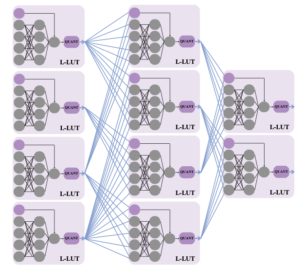
A key question in the various LUT-based machine learning frameworks we have introduced, is how to parameterise the space of the functions implemented in the LUTs. Our first work in this area, LUTNet, with my former PhD student Erwei Wang (now with AMD), took a fully general approach: if you want to learn a $K$ -input Boolean function, then learn all $2^K$ lines in that function’s truth table. Since then, Marta and I have been exploring ways of parameterising that space to decouple the complexity of the function-classes implemented from the number of inputs. This gave rise to PolyLUT (parameterised as polynomials) and NeuraLUT (parameterised as small neural networks). 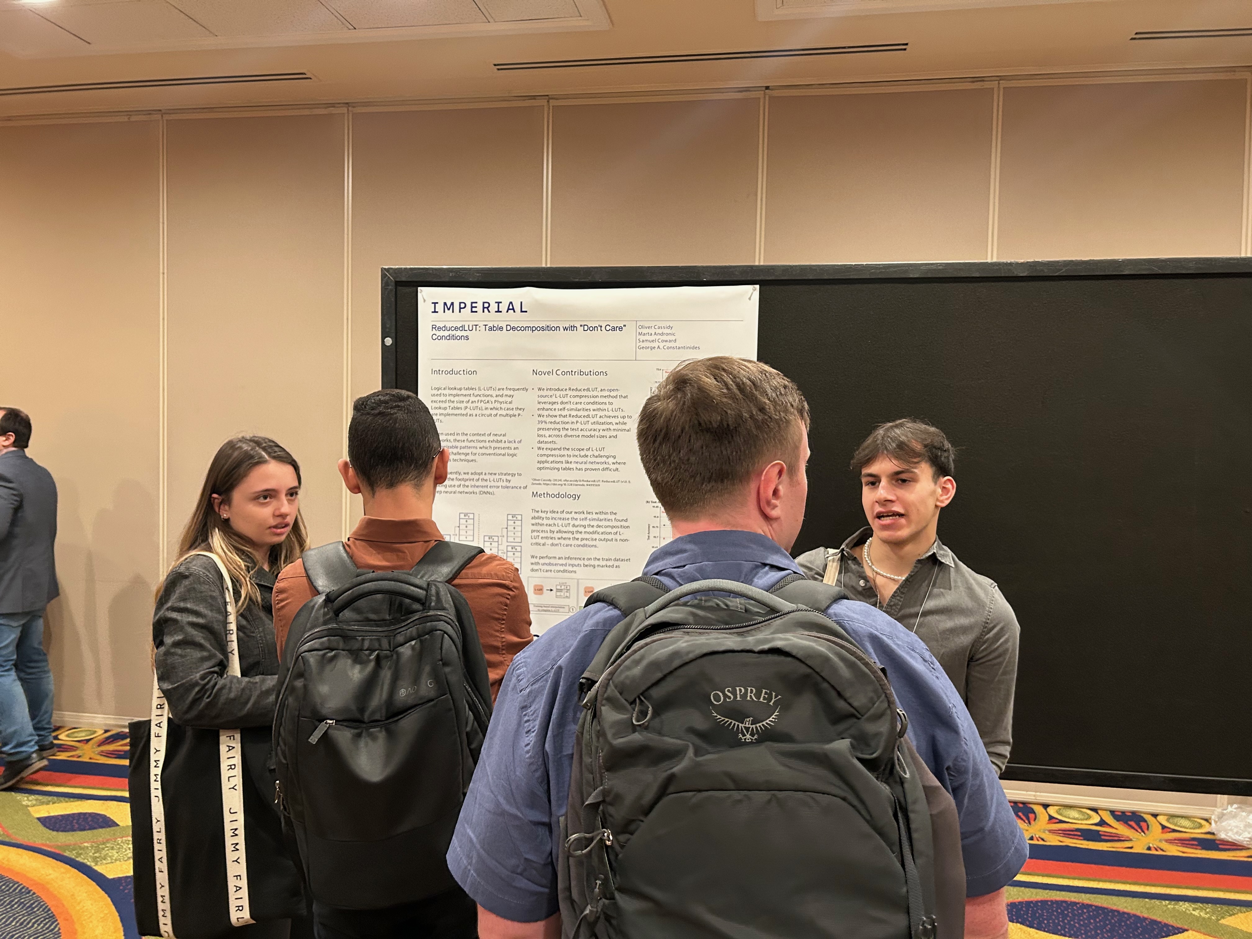Once we have learnt a function $f$ , all these methods enumerate the inputs of the function for the discrete space of quantised activations to produce the L-LUT. Olly’s work introduces `don’t cares’ into the picture: if a particular combination of inputs to the function is never, or rarely, seen in the training data, then the optimisation is allowed to treat the function as a don’t care at that point.

Olly picked up CompressedLUT from Khataei and Bazargan, and investigated the injection of don’t care conditions into their decomposition process. The results are quite impressive: up to a 39% drop in the P-LUTs (area) required to implement the L-LUTs, with near zero loss in classification accuracy of the resulting neural network.

To my mind, one of the most interesting aspects of Olly’s summer work is the observation that aggressively targeting FPGA area reduction through don’t care conditions without explicitly modelling the impact on accuracy, nevertheless has a negligible or even a positive impact on test accuracy. This can be interpreted as a demonstration that (i) the generalisation capability of the LUT-based network is built into the topology of the NeuraLUT network and (ii) that, in line with Occam’s razor, simple representations – in this case, simple circuits – generalise better.

Our group is very proud of Olly!

NeuraLUT: Networks inside LUTs

In early September, my PhD student Marta Andronic will be off to Turin to present our latest work “NeuraLUT: Hiding Neural Network Density in Boolean Synthesizable Functions” at the Field-Programmable Logic and Applications conference. Ahead of the detailed presentation at the conference, this blog post provides a short accessible summary of her exciting work.

In 2019 I first proposed making better use of FPGA lookup tables by exposing them as trainable hardware, together with my then PhD student Erwei Wang and coauthors, in our LUTNet work. In common with AMD’s LogicNets and our PolyLUT, our new work NeuraLUT hides certain aspects of a neural network within a synthesisable Boolean lookup table (which we call an L-LUT), to achieve very efficient and very low latency inference. LogicNets hid a dot product and activation function – the clever thing in LogicNets was that, as a result, the weights can be real-valued – no quantisation needs to be performed, because the only thing that’s important is the finite truth table of the lookup table; once this has been enumerated, the real-valued weights are irrelevant, the only quantisation is at the inputs and outputs of the L-LUT. The tradeoff here is that LogicNets networks needed to be extremely sparse.

NeuraLUT takes this a step beyond by hiding whole neural networks inside Boolean lookup tables! These internal neural networks can be fully dense – or even irregularly connected – and real-valued in both weight and activation, for the same reason. The only thing that’s important is that the inputs and outputs of these “sub networks” are quantised and connections between sub networks are sparse, because these are the only parts that get exposed to the hardware design itself. One can interpret the resulting network as a standard deep neural network, with a specific hardware-friendly sparsity pattern, as illustrated in the figure below.

The increased expressive power of NeuraLUT leads to considerable reductions in latency. We’re targeting here very low latency applications like you may find in particle physics. 12 nanosecond MNIST classification, anyone? 3 nanoseconds to tag jet substructures in a particle accelerator? Come and listen to Marta’s talk to find out how!