FCCM 2025

I’ve recently returned from the IEEE International Symposium on Field-Programmable Custom Computing Machines (known as FCCM). I used to attend FCCM regularly in the early 2000s, and while I have continued to publish there, I have not attended myself for some years. I tried a couple of years ago, but ended up isolated with COVID in Los Angeles. In contrast, I am pleased to report that the conference is in good health!

The conference kicked off on the the evening of the 4th May, with a panel discussion on the topic of “The Future of FCCMs Beyond Moore’s Law”, of which I was invited be be part, alongside industrial colleagues Chris Lavin and Madhura Purnaprajna from AMD, Martin Langhammer from Altera, and Mark Shand from Waymo. Many companies have tried and failed to produce lasting post-Moore alternatives to the FPGA and the microprocessor over the decades I’ve been in the field and some of these ideas and architectures (less commonly, associated compiler flows / design tools) have been very good. But, as Keynes said, “markets can remain irrational longer than you can remain solvent”. So instead of focusing on commercial realities, I tried to steer the panel discussion towards the genuinely fantastic opportunities our academic field has for a future in which power, performance and area innovation changes become a matter of intellectual advances in architecture and compiler technology rather than riding the wave of technology miniaturisation (itself, of course, the product of great advances by others).
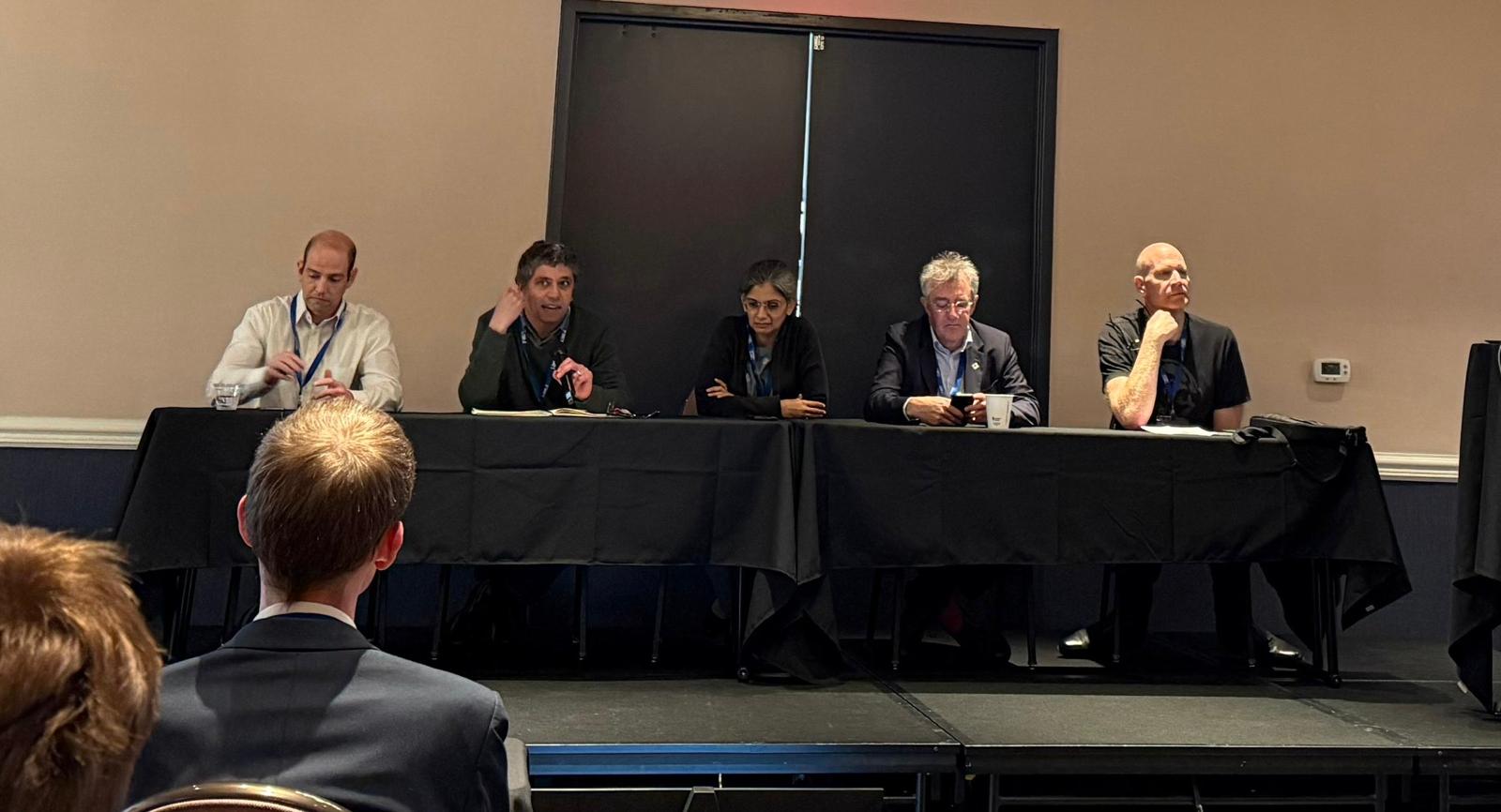
The following day, the conference proper kicked off. Some highlights for me from other authors included the following papers aligned with my general interests:

  • AutoNTT: Automatic Architecture Design and Exploration for Number Theoretic Transform Acceleration on FPGAs from Simon Fraser University, presented by Zhenman Fang.
  • RealProbe: An Automated and Lightweight Performance Profiler for In-FPGA Execution of High-Level Synthesis Designs from Georgia Tech, presented by Jiho Kim from Callie Hao‘s group.
  • High Throughput Matrix Transposition on HBM-Enabled FPGAs from the University of Southern California (Viktor Prasanna‘s group).
  • ITERA-LLM: Boosting Sub-8-Bit Large Language Model Inference Through Iterative Tensor Decomposition from my colleague Christos Bouganis‘ group at Imperial College, presented by Keran Zheng.
  • Guaranteed Yet Hard to Find: Uncovering FPGA Routing Convergence Paradox from Mirjana Stojilovic‘s group at EPFL – and winner of this year’s best paper prize!

In addition, my own group had two full papers at FCCM this year:

  • Banked Memories for Soft SIMT Processors, joint work between Martin Langhammer (Altera) and me, where Martin has been able to augment his ultra-high-frequency soft-processor with various useful memory structures. This is probably the last paper of Martin’s PhD – he’s done great work in both developing a super-efficient soft-processor and in forcing the FPGA community to recognise that some published clock frequency results are really quite poor and that people should spend a lot longer thinking about the physical aspects of their designs if they want to get high performance.
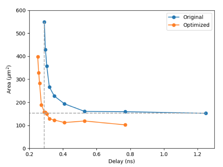
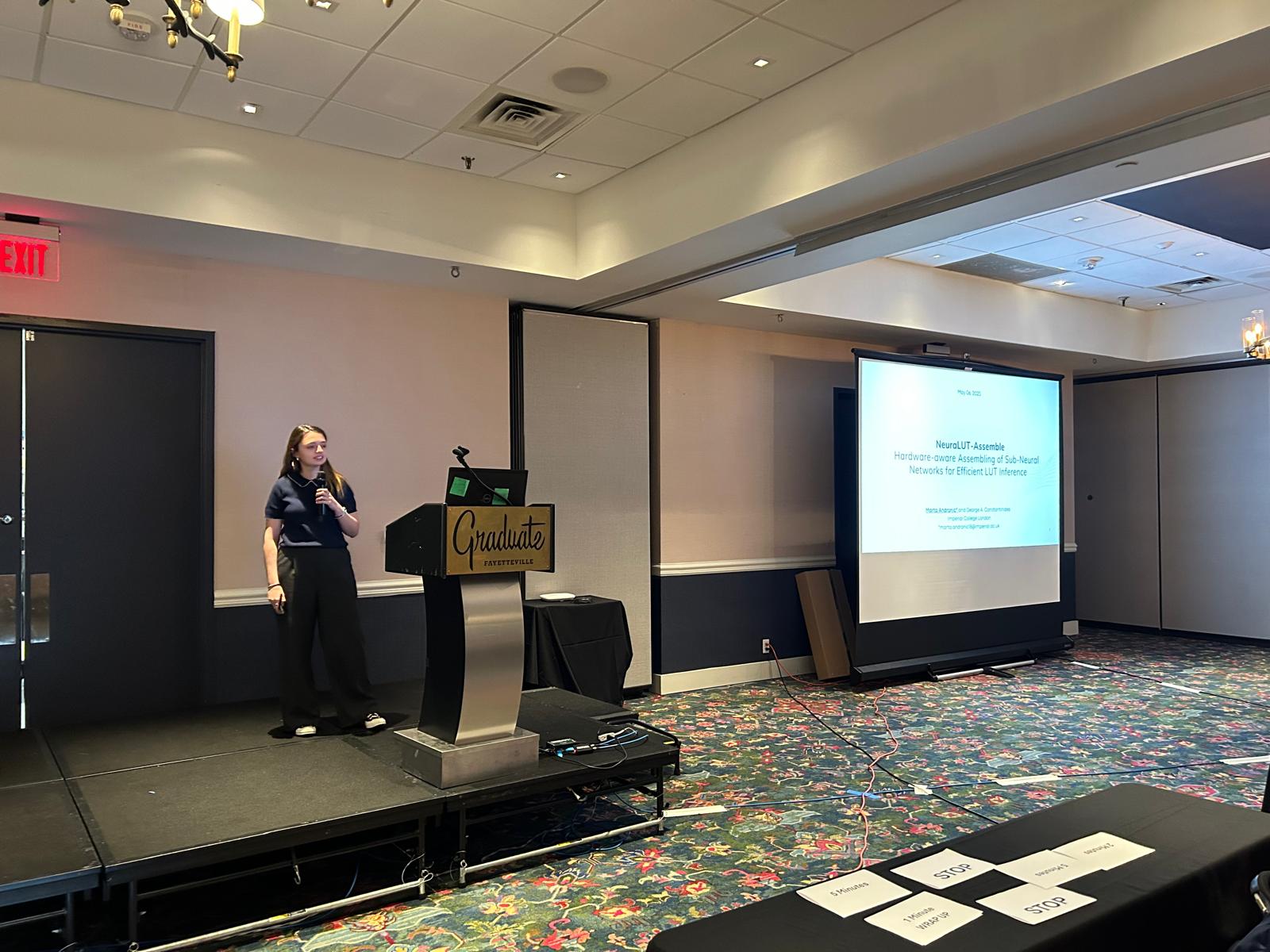
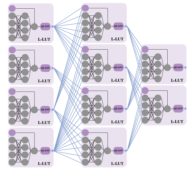
  • NeuraLUT-Assemble: Hardware-aware Assembling of Sub-Neural Networks for Efficient LUT Inference, joint work between my PhD student Marta Andronic and me. I think this is a landmark paper in terms of the results that Marta has been able to achieve. Compared to her earlier NeuraLUT work which I’ve blogged on previously, she has added a way to break down large LUTs into trees of smaller LUTs, and a hardware-aware way to learn sparsity patterns that work best, localising nonlinear interactions in these neural networks to within lookup tables. The impact of these changes on the area and delay of her designs is truly impressive.
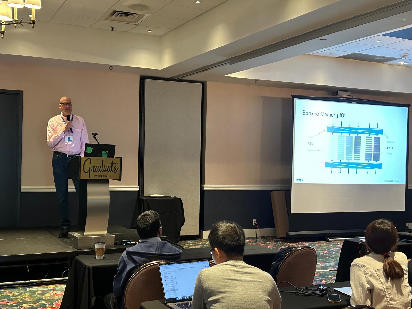
Overall, it was well worth attending. Next year, Callie will be hosting FCCM in Atlanta.

Machine Learning with Large Lookup Tables

Readers of this blog will know that I have been interested in how to bridge the worlds of Boolean logic and machine learning, ever since I published a position paper in 2019 arguing that this was the key to hardware-efficient ML.

Since then, I have been working on these ideas with several of my PhD students and collaborators, most recently my PhD student Marta Andronic‘s work forms the leading edge of the rapidly growing area of LUT-based neural networks (see previous blog posts). Central to both Marta’s PolyLUT and NeuraLUT work (and also LogicNets from AMD/Xilinx) is the idea that one should train Boolean truth tables (which we call L-LUTs for logical LUTs) which then, for an FPGA implementation, get mapped into the underlying soft logic (which we call P-LUTs, for physical LUTs).

Last Summer, Marta and I had the pleasure of supervising a bright undergraduate student at Imperial, Olly Cassidy, who worked on adapting some ideas for compressing large lookup tables coming out of the lab of my friend and colleague Kia Bazargan, together with his student Alireza Khataei at the University of Minnesota, to our setting of efficient LUT-based machine learning. Olly’s paper describing his summer project has been accepted by FPGA 2025 – the first time I’ve had the pleasure to send a second-year undergraduate student to a major international conference to present their work! In this blog post, I provide a simple introduction to Olly’s work, and explain my view of one of the most interesting aspects, ahead of the conference.

A key question in the various LUT-based machine learning frameworks we have introduced, is how to parameterise the space of the functions implemented in the LUTs. Our first work in this area, LUTNet, with my former PhD student Erwei Wang (now with AMD), took a fully general approach: if you want to learn a K-input Boolean function, then learn all 2^K lines in that function’s truth table. Since then, Marta and I have been exploring ways of parameterising that space to decouple the complexity of the function-classes implemented from the number of inputs. This gave rise to PolyLUT (parameterised as polynomials) and NeuraLUT (parameterised as small neural networks). Once we have learnt a function f, all these methods enumerate the inputs of the function for the discrete space of quantised activations to produce the L-LUT. Olly’s work introduces `don’t cares’ into the picture: if a particular combination of inputs to the function is never, or rarely, seen in the training data, then the optimisation is allowed to treat the function as a don’t care at that point.

Olly picked up CompressedLUT from Khataei and Bazargan, and investigated the injection of don’t care conditions into their decomposition process. The results are quite impressive: up to a 39% drop in the P-LUTs (area) required to implement the L-LUTs, with near zero loss in classification accuracy of the resulting neural network.

To my mind, one of the most interesting aspects of Olly’s summer work is the observation that aggressively targeting FPGA area reduction through don’t care conditions without explicitly modelling the impact on accuracy, nevertheless has a negligible or even a positive impact on test accuracy. This can be interpreted as a demonstration that (i) the generalisation capability of the LUT-based network is built into the topology of the NeuraLUT network and (ii) that, in line with Occam’s razor, simple representations – in this case, simple circuits – generalise better.

Our group is very proud of Olly!

NeuraLUT: Networks inside LUTs

In early September, my PhD student Marta Andronic will be off to Turin to present our latest work “NeuraLUT: Hiding Neural Network Density in Boolean Synthesizable Functions” at the Field-Programmable Logic and Applications conference. Ahead of the detailed presentation at the conference, this blog post provides a short accessible summary of her exciting work.

In 2019 I first proposed making better use of FPGA lookup tables by exposing them as trainable hardware, together with my then PhD student Erwei Wang and coauthors, in our LUTNet work. In common with AMD’s LogicNets and our PolyLUT, our new work NeuraLUT hides certain aspects of a neural network within a synthesisable Boolean lookup table (which we call an L-LUT), to achieve very efficient and very low latency inference. LogicNets hid a dot product and activation function – the clever thing in LogicNets was that, as a result, the weights can be real-valued – no quantisation needs to be performed, because the only thing that’s important is the finite truth table of the lookup table; once this has been enumerated, the real-valued weights are irrelevant, the only quantisation is at the inputs and outputs of the L-LUT. The tradeoff here is that LogicNets networks needed to be extremely sparse.

NeuraLUT takes this a step beyond by hiding whole neural networks inside Boolean lookup tables! These internal neural networks can be fully dense – or even irregularly connected – and real-valued in both weight and activation, for the same reason. The only thing that’s important is that the inputs and outputs of these “sub networks” are quantised and connections between sub networks are sparse, because these are the only parts that get exposed to the hardware design itself. One can interpret the resulting network as a standard deep neural network, with a specific hardware-friendly sparsity pattern, as illustrated in the figure below.

The increased expressive power of NeuraLUT leads to considerable reductions in latency. We’re targeting here very low latency applications like you may find in particle physics. 12 nanosecond MNIST classification, anyone? 3 nanoseconds to tag jet substructures in a particle accelerator? Come and listen to Marta’s talk to find out how!

Open Source MX Library

Readers of this blog may be aware that several key industrial players recently released the MX standard for low-precision computation, mainly targeting its use in machine learning. I reviewed the standard in an earlier blog post.

I’m pleased to report that my PhD student Ebby Samson has released an open source RTL hardware implementation of the key operators from the standard. In joint work with Naveen Mellempudi from AMD, Wayne Luk from Imperial and myself, he describes the library in our forthcoming paper at the International Conference on Field-Programmable Logic and Applications. If you will be in Turin in early September, please come and hear Ebby talking about his work.

The library supports all the concrete formats in the standard and more besides. Ebby has also released an extension to the AMD Brevitas quantisation-aware training PyTorch library that lets you train your models with eventual MX implementation in mind.

Please do read our paper, integrate our hardware designs into your work, and use our Brevitas library to do your neural network training! Links to all in the paper.

Energy: Rewriting the Possibilities

In early June, my PhD student Sam Coward (co-advised by Theo Drane from Intel), will travel to ARITH 2024 in Málaga to present some of our most recent work, “Combining Power and Arithmetic Optimization via Datapath Rewriting”, a joint paper with Emiliano Morini, also of Intel. In this blog post, I will describe the fundamental idea of our work.

It’s well-known that ICT is driving a significant amount of energy consumption in the modern world. The core question of how to organise the fundamental arithmetic operations in a computer in order to reduce power (energy per unit time) has been studied for a long time, and continues to be a priority for designers across industry, including the group at Intel with whom this work has been conducted.

Readers of this blog will know that Sam has been doing great work on how to explore the space of behaviourally equivalent hardware designs automatically. First for area, then for performance, and now for power consumption!

In our latest work, Sam looks at how we can use the e-graph data structure, and the related egg tool, to tightly integrate arithmetic optimisations (like building multi-input adders in hardware) with clock gating and data gating, two techniques for power saving. Clock gating avoids clocking new values into registers in hardware if we know they’re not going to be used in a given cycle; this avoids the costly switching activity associated with propagating unused information in a digital circuit. Data gating also avoids switching, but in a different way – by replacing operands with values inducing low switching: for example, if I do not end up using a result of a \times b, then I may as well be computing a \times 0. In both cases, the fundamental issue becomes how to identify whether a value will be unused later in a computation. Intriguingly, this question is tightly related to the way a computation is performed: there are many ways of computing a given mathematical computation, and each one will have its own redundancies to exploit.

In our ARITH 2024 paper, Sam has shown how data gating and clock gating can be expressed as rewrites over streams of Boolean data types, lifting our previous work that looks at equivalences between bit vectors, to equivalences over streams of bit vectors. In this way, he’s able to express both traditional arithmetic equivalences like a + (b + c) = (a + b) + c and equivalences expressing clock and data gating within the same rewriting framework. A collection of these latter equivalences are shown in the table below from our paper.

Some of the rewrites between equivalent expressions used in our ARITH 2024 paper

Sam has been able to show that by combining the rewrites creatively, using arithmetic rewrites to expose new opportunity for gating, our tool ROVER is able to save some 15% to 30% of power consumption over a range of benchmark problems of industrial interest. Moreover, ROVER will automatically adjust the whole design to better suit different switching profiles, knowing that rarely-switching circuit components are less problematic for energy, and prioritising exposing rewrites where they are needed.

I think this is really interesting work, and shows just how general the e-graph approach to circuit optimisation can be. If you’re going to ARITH 2024, do make sure to talk to Sam and find out more. If not, make sure to read his paper!

PolyLUT: Ultra low latency inference

This week my PhD student Marta Andronic will present our paper “PolyLUT: Learning Piecewise Polynomials for Ultra-Low Latency FPGA LUT-based Inference” at the International Conference on Field Programmable Technology (FPT), in Yokohama, Japan, where it has been short-listed for the best paper prize. In this blog post I hope to provide an accessible introduction to this exciting work.

FPGAs are a great platform for high-performance (and predictable performance) neural network inference. There’s a huge amount of work that’s gone into both the architecture of these devices and into the development of really high quality logic synthesis tools. In our work we look afresh at the question of how to best leverage both of these in order to do really low-latency inference, inspired by the use of neural networks in environments like CERN, where the speed of particle physics experiments and the volume of data generated demands really fast classification decisions: “is this an interesting particle interaction we’ve just observed?”

Our colleagues at Xilinx Research Labs (now part of AMD) published a great paper called LogicNets in 2020 that aimed to pack the combination of linear computation and activation function in a neural network into lookup tables in Verilog, a hardware description language, which then get implemented using the logic synthesis tools on the underlying soft-logic of the FPGA. Let’s be a bit more precise. The operation of a typical neuron in an artificial neural network is to compute the real-valued function y = \phi( w^T x + b ) for its inputs x and some learned weight vector w and bias b, where \phi is typically a fixed nonlinear function such as a ReLU. In practice, of course we use finite precision approximations to x and y. The Xilinx team noted that if they restrict the length of the vector x to be small enough, then the quantised version of this entire function can be implemented by simply enumerating all possible values of the input vector x to form a truth table for y, and using the back-end logic synthesis tools to implement this function efficiently, stitching together the neurons constructed in this way to form a hardware neural network. Moreover, note that in this setting one does not need to quantise the weights and bias at all – since the computation is absorbed in a truth table, arbitrary real-valued weights are just fine.

Marta and I have generalised this approach considerably. Firstly, we note that once we’re down at the level of enumerating truth tables, there’s no particular reason to limit ourselves to functions of the form y = \phi( w^T x + b ) – why not use an arbitrary function instead? From the perspective of the enumeration process and logic synthesis, it makes no difference. But from the perspective of neural network training, it certainly does. If we really wanted to look at arbitrary functions, we’d need a number of parameters to train that scales exponentially with the number of bits used to represent the entire vector x. This might be OK for very small vectors – indeed, with my former student Erwei Wang, I looked at something similar for the tiny physical lookup tables inside FPGA devices – but at the scale of neurons this is infeasible. So what family of functions should we use? Marta and I propose to use polynomials, where the total degree is fixed as a user-defined parameter we call D. In this way, we can tune a knob: turn down to D=1 for minimal expressivity but the smallest number of parameters to train, and recover LogicNets as a special case; turn up D and you get much more expressive functions you can pack into your LUTs, at the cost of more parameters to train. In a classical neural network, composition of linear layers and ReLU functions gives rise to the overall computation of a continuous piecewise linear function. In our networks, we have continuous piecewise polynomial functions. The important thing, though, is that we never have to do all the expensive multiplications and additions one typically associates with evaluating a polynomial – the implementation is all just a table lookup for each neuron, just like in the linear case.

So what does higher degree actually buy us? It’s well known that deep neural networks of the classical form are universal function approximators, so with enough neurons (enough depth or width), we can arbitrarily closely approximate a continuous function anyway. But by packing in more functionality into each neuron, which anyway gets enumerated and implemented using lookup tables in the FPGA (just like the classical case), we can get the same accuracy with fewer layers of network. And fewer layers of network means fewer layers of Boolean logic, which means lower latency. In fact, we show in our results that one can often at least halve the latency by using our approach: we run 2x as fast! This two-fold speedup comes from the more intricate decision boundaries one can implement with polynomial compute; look at this beautiful near-separation of the two dot colours using a curved boundary, and imagine how many small linear segments you would need to do a similar job – this provides the intuition for just why our networks perform so well.

PolyLUT is available for others to use and experiment with. Don’t just take our word for it, download Marta’s code and try it out for yourself! I’m also delighted that Marta’s paper at FPT is one of just three at the conference to have earned all available ACM badges, verifying that not only is her work public, but it has been independently verified as reproducible. Thank you to the artifact review team for their work on the verification!

Supercharging Formal with E-Graphs

Designing circuits is not easy. Mistakes can be made, and mistakes made are not easily fixed. Even leaving aside safety-critical applications, product recalls can cost upwards of hundreds of millions of US$, and nobody wants to be responsible for that. As a result, the industry invests a huge effort in formally verifying hardware designs, that is coming up with computer-generated or computer-assisted proofs of hardware correctness.

My Intel-funded PhD student Sam Coward (jointly advised by Theo Drane) is about to head off to FMCAD 2023 in Ames, Iowa, to present a contribution to making this proof generation process speedier and more automated, while still relying on industry-standard tried and trusted formal verification tools. Together with his Intel colleague Emiliano Morini and then-intern (and Imperial student) Bryan Tan, Sam noticed that the e-graph techniques we have been using in his PhD for optimising datapath [1, 2] also have a natural application to verifying datapath designs, akin – but distinct – to their long-time use as a data-structure in SMT solvers.

The basic idea is straight-forward. Ever since our earliest ARITH paper, we’ve developed a toolbox of Intel-inspired rewrite rules that can be applied to optimise designs across parametric bitwidths. Our optimisation flow, called ROVER, applies these to a single expression we wish to optimise, and then we extract a minimal cost implementation. Our new paper asks a different question: what if we start, not from a single expression we wish to optimise, but from two expressions we’re trying to prove to be equivalent?

Following the approach I blogged about here from ROVER, if the expressions are not equivalent then they should never end up in the same equivalence class after multiple rewrite iterations. If they are equivalent then they may or may not end up in the same equivalence class: we provide no guarantees of completeness. So let’s think about what happens in each of these cases.

If they end up in the same equivalence class, then our tool thinks it has proven the two expressions to be equivalent. But no industrial design team will trust our tool to just say so – and rightly so! – tool writers make mistakes too. However, work by Sam and other colleagues from the Universities of Washington and Utah, has provided a methodology by which we can use our tool’s reasoning to export hints, in the form of intermediate proof steps, to a trusted industrial formal verification tool. And so this is how we proceed: our tool will generate many, sometimes hundreds, of hints which will help state-of-the-art industrial formal verification tools to find proofs more quickly – sometimes much more quickly – than they were able to do so beforehand.

So what if the two expressions don’t end up in the same equivalence class, despite actually being equivalent? No problem! We can still find two expressions for which their proof of equivalence, via some external tool, makes the overall proof we’re aiming for much easier… crunching down the proof to its hard essence, stripping away what we can. The main technical idea here is how to extract the expressions from the e-graph. Rather than aiming for the best possible implementation cost, as we did with ROVER, we aim to minimise the distance between the two implementations that are left for the industrial tool to verify. The overall process is shown in the figure below, where “EC” refers to an equivalence check conducted by the industrially-trusted tool and S^* and I^* are the extracted “close” expressions.

We show one example where, without the hints provided by our tool, the industrial formal verifier does not complete within a 24 hour timeout. Even when results are achievable with the industrial formal verifier, we still get an up to a 6x speedup in proof convergence.

This work forms a really nice “power use” of e-graphs. If you are at FMCAD 2023, come along and hear Sam talk about it in person!

Discovering Special Cases

My PhD student Sam Coward (jointly advised by Theo Drane from Intel) is about to head off on a speaking tour, where he will be explaining some of our really exciting recent developments. We’ve developed an approach that allows the discovery, exploitation, and generation of datapath hardware that works well in certain special cases. We’ve developed some theory (based on abstract interpretation), some software (based on egg), and some applications (notably in floating-point hardware design). Sam will be formally presenting this work at SOAP, EGRAPHS, and DAC over the coming weeks. In this blog post, I will try to explain the essence of the work. More detail can be found in the papers, primarily [1,2], with [3] for background.

We know that sometimes we can take shortcuts in computation. As a trivial example, we know that \text{abs}(x) can just be replaced by x for non-negative values of x. Special cases abound, and are often used in complex ways to create really efficient hardware. A great example of this is the near/far-path floating-point adder. Since the publication of this idea by Oberman and Flynn in the late 1990s, designs based on this have become standard in modern hardware. These designs use the observation that there are two useful distinct regimes to consider when adding two values of differing sign. If the numbers are close in magnitude then very little work has to be done to align their mantissas, yet a lot of work might be required to renormalise the result of the addition. On the other hand, if the two numbers are far in magnitude then a lot of work might be needed to align their mantissas, yet very little is required to renormalise the result of the addition. Thus we never see both alignment and renormalisation being significant computational steps.

Readers of this blog may remember that Sam, Theo and I published a paper at ARITH 2022 that demonstrated that e-graphs can be used to discover hardware that is equivalent in functionality, but better in power, performance, and area. E-graphs are built by repeatedly using rewrite rules of the form \ell \to r, e.g. \texttt{x + x} \to \texttt{2*x}. But our original ARITH paper wasn’t able to consider special cases. What we really need for that is some kind of conditional rewrite rules, e.g. x \geq 0 \Rightarrow \texttt{abs(x)} \to \texttt{x}, where I am using math script to denote the value of a variable and teletype script to denote an expression.

So we set out to answer:

  1. how can we deal with conditional rewrites in our e-graphs?
  2. how can we evaluate whether a condition is true in a certain context?
  3. how can we make use of this to discover and optimise special cases in numerical hardware?

Based on an initial suggestion from Pavel Panchekha, Sam developed an approach to conditionality by imagining augmenting the domain in which we’re working with an additional element, let’s call it *. Now let’s imagine introducing a new operator \texttt{assume} that takes two expressions, the second of which is interpreted as a Boolean. Let’s give \texttt{assume} the following semantics: \llbracket \texttt{assume(x,c)} \rrbracket = \llbracket \texttt{x} \rrbracket \text{ if } \llbracket c \rrbracket \text{ , and } * \text{, otherwise}. In this way we can ‘lift’ equivalences in a subdomain to equivalences across the whole domain, and use e-graphs without modification to reason about these equivalences. Taking the absolute value example from previously, we can write this equivalence as \texttt{assume( abs(x), x >= 0 )} \to \texttt{assume( x, x >= 0 )}. These \texttt{assume} function symbols then appear directly within the e-graph data structure. Note that the assume on the right-hand side here is important: we need both sides of the rewrite to evaluate to the same value for all possible values of x, and they do: for negative values they both evaluate to * and for non-negative values they both evaluate to x.

So how do we actually evaluate whether a condition is true in a given context? This is essentially a program analysis question. Here we make use of a variation of classical interval arithmetic. However, traditionally interval arithmetic has been a fairly weak program analysis method. As an example, if we know that x \in [-1,1], then a classical evaluation of x - x would give me [-2,2], due to the loss of information about the correlation between the left and right-hand sides of the subtraction operator. Once again, our e-graph setting comes to the rescue! Taking this example, a rewrite \mathtt{x - x} \to \mathtt{0} would likely fire, resulting in zero residing in the same e-class as \mathtt{x - x}. Since the interval associated with \mathtt{0} is [0,0], the same interval will automatically be associated with \mathtt{x - x} by our software, leading to a much more precise analysis.

This interaction between rewrites and conditions goes even further: a more precise analysis leads to the possibility to fire more conditional rewrite rules, as more conditions will be known to hold; firing more rewrite rules results in an even more precise analysis. The two techniques reinforce each other in a virtuous cycle:

A virtuous cycles: greater precision leads to more rewrites leads to greater precision.

Our technique is able to discover, and generate RTL for, near/far-path floating-point adders from a naive RTL implementation (left transformed to right, below), resulting in a 33% performance advantage for the hardware.

Left: A naive floating-point subtractor. Right: The subtractor produced by our software.

I’m really excited by what Sam’s been able to achieve, as I really think that this kind of approach has the potential to lead to huge leaps forward in electronic design automation for word-level designs.

Put Your Resource Where it’s Needed!

We all know that we have finite resources to accomplish a variety of tasks. Some tasks are easier than others, so we tend to spend less time and energy on them. Yet – when we survey the landscape of traditional neural networks – this observation does not apply to them. Take a convolutional neural network classifying pictures: does it do any less work (floating point operations, perhaps) if the picture is “obviously a cat” than if it’s a “cat hiding in the bushes”? Traditionally, the answer is a clear “no”, because there is no input dependence in the control-flow of the inference algorithm: every single image is processed in exactly the same way and takes exactly the same work.

But there are people who have looked to address this fundamental shortcoming by designing algorithms that put in less work if possible. Chief amongst these techniques is an approach known as “early exit neural networks”. The idea of these networks is that the network itself generates a confidence measure: if it’s confident early on, then it stops computing further and produces an early result.

My student Ben Biggs (jointly advised by Christos Bouganis) has been exploring the implications of bringing FPGAs to automatically accelerate such networks. There exist several good tool flows (e.g. fpgaConvNet, HPIPE) for automatically generating neural network implementations on FPGAs, but to the best of our knowledge, none of them support such dynamic control flow. Until now. Next week at FCCM 2023, Ben will be presenting our paper ATHEENA: A Toolflow for Hardware Early-Exit Network Automation.

The basic idea of ATHEENA is that early exit networks come in chunks, each of which is utilised a certain proportion of the time (e.g. 10% of images are hard to classify, 90% are not). So we make use of an existing neural network generator to generate each chunk, but allocate different FPGA resources to the different parts of the network, in order to maintain a steady throughput with no back pressure build-up points in the inference pipeline.

This principle is illustrated below. Imagine that the first stage of a network executes no matter what the input. Then I can create a throughput / area Pareto curve shown on the top left. Equally, I can create a throughput / area Pareto curve for the second stage, and then scale up the throughput achievable by a function of how frequently I actually need to use that stage: if it’s only needed 10% of the time, then I can support a classification rate 10x higher than the nominal throughput of the design returned by a standard DNN generator. By combining these two throughput / area curves for the same nominal throughput, I get an allocation of resources to each part of the network. Of course, if the nominal proportion p 
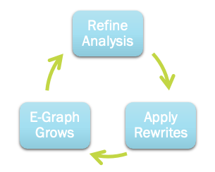
of ‘hard’ samples I used to characterise the network varies in practice from the actual proportion q, then I may end up with a somewhat different behaviour, as indicated by the purple region.

In practice, it turns out that this works really well. The graph below from Ben’s paper shows that on a real example, running on a real FPGA board, he’s able to improve throughput by more than 2x for the same area or reduce area by more than half for the same throughput.

I’m delighted that Ben’s work has been nominated for the best paper prize at FCCM this year and that it has received all three reproducibility badges available: Open Research Objects, Research Objects Reviewed and Results Reproduced, indicating Ben’s commitment to high quality reproducible research in our field.

If you plan to be in Los Angeles next week, come and hear Ben talk about it!

Equivalent. But better.

Ever since primary (elementary) school, we’ve known that multiplying an integer by 10 is easy. No need for the long written calculations we churn through when doing multiplication by hand. Just stick an extra zero on the end, and we’re done. Multiplication is (relatively) hard, concatenation of digits is easy. And yet, in this case, they’re equivalent in terms of the operation they perform.

Similar equivalences abound in the design of digital hardware for arithmetic computation, and my PhD student Sam Coward (jointly supervised by Theo Drane from Intel) has been devising ways to automatically take advantage of such equivalences to make Intel hardware smaller and more efficient. He will be presenting our work on this topic at the main computer arithmetic conference, ARITH, next week. The conference will be online, and registration is free: https://arith2022.arithsymposium.org.

Let’s explore this example from our early school years a bit more. I’ll use Verilog notation \{\cdot,\cdot\} 
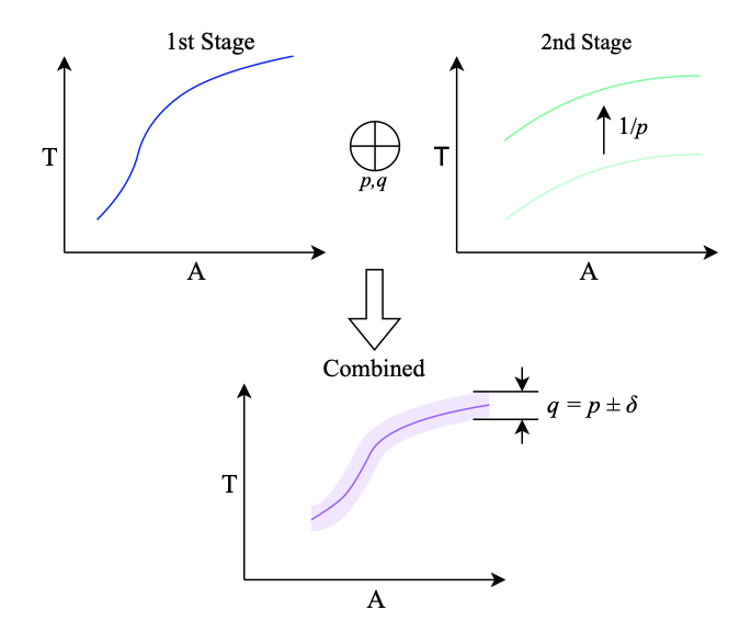
to denote a function taking two bit vectors and concatenating them together. Of course the ‘multiplication by 10 is easy’ becomes ‘multiplication by 2 is easy’ in binary. Putting this together, we can write 2*x \simeq \{x,0\}, meaning that multiplication by two is the same as concatenation with a zero. But what does ‘the same as’ actually mean here? Clearly they are not the same expression syntactically and one is cheap to compute whereas one is expensive. What we mean is that no matter which value of x I choose, the value computed on the left hand side is the same as the value computed on the right hand side. This is why I’ve chosen to write \simeq rather than =. \simeq clearly defines a relation on the set of expressions. This is a special kind of relation called a congruence: it’s an equivalence relation, i.e. it is symmetric, transitive, and reflexive, but it also ‘plays well’ with function application: if x \simeq y then it necessarily follows that f(x) \simeq f(y) for every function symbol f. Like any equivalence relation on a set, \simeq partitions the set into a set of equivalence classes: in our setting a class corresponds to expressions that can be freely interchanged without changing the functionality of our hardware, even if it changes the performance, area or energy consumption of the resulting design.

Our colleagues Willsey, Nandi, Wang, Flat, Tatlock and Panchekha recently published egg, a wonderful open source library for building and exploring data structures known as ‘e-graphs’, specifically designed to capture these relations on expressions. Sam, Theo and I have developed a set of ‘rewrites’ capturing some of the important intuition that Intel designers apply manually, and encoded these for use within egg. To give you a flavour of these rewrites, here’s the table from Sam’s paper; you can see the example we started with is hiding in there by the name ‘Mult by Two’. The subscripts are used to indicate how many digits we’re dealing with; not all these rules are true for arbitrarily-sized integers, and Sam has gone to some lengths to discover simple rules – listed here as ‘sufficient condition’ – for when they can be applied. This is really important in hardware, where we can use as few or as many bits as the job requires.

You can imagine that, when you have this many equivalences, they all interact and you can very quickly build up a very large set of possible equivalent expressions. e-graphs help us to compactly represent this large set.

Once our tool has spent enough time building such a representation of equivalences, we need to extract an efficient implementation as a hardware implementation. This is actually a hard problem itself, because common subexpressions change the hardware cost. For example if I’m calculating (x+1)*(x+1) 
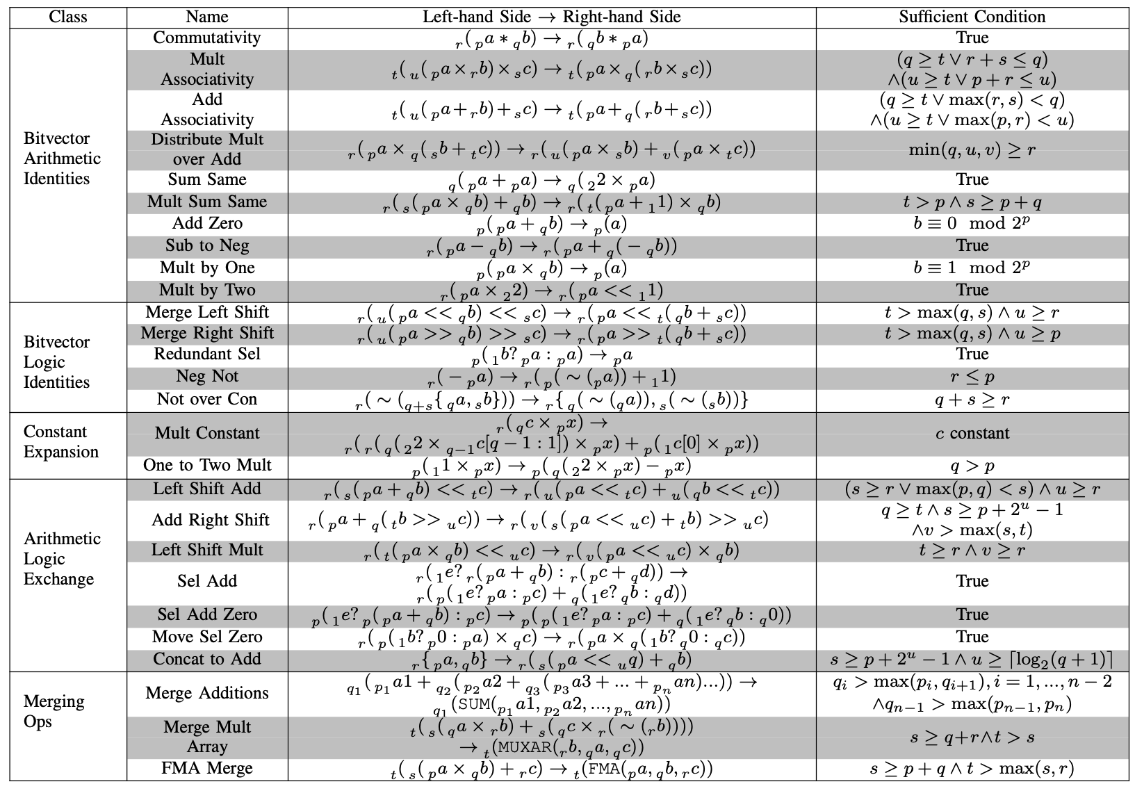
then I wouldn’t bother to calculate x+1 twice. We describe in our paper how we address this problem via an optimisation formulation. Our tool solves this optimisation and produces synthesisable Verilog code for the resulting circuit.

So, does it generate good circuits? It certainly does! The graph below shows the possible circuit area and performance achievable before (blue) and after (orange) the application of our tool flow before standard logic synthesis tools. For this example, silicon area can be reduced by up to around 70% – a very significant saving.

Area/Delay tradeoff for a smoothing kernel before and after our work

I’ve really enjoyed working on this topic with Sam and Theo. Lots more exciting content to follow. In the meantime, please tune in to hear Sam talk about it next week.