Neural Networks, Approximation and Hardware

My PhD student Erwei Wang, various collaborators and I have recently published a detailed survey article on this topic: Deep Neural Network Approximation for Custom Hardware: Where We’ve Been, Where We’re Going, to appear in ACM CSUR. In this post, I will informally explain my personal view of the role of approximation in supervised learning (classification), and how this links to the very active topic of DNN accelerator design in hardware.

We can think of a DNN as a graph $G$ , where nodes perform computations and edges carry data. This graph can be interpreted (executed) as a function $\llbracket G \rrbracket$ mapping input data to output data. The quality of this DNN is typically judged by a loss function $\ell$ . Let’s think about the supervised learning case: we typically evaluate the DNN on a set of $n$ test input data points $x_i$ and their corresponding desired output $y_i$ , and compute the mean loss:

$L(G) = \frac{1}{n} \sum_{i=1}^n {\ell\left( \llbracket G \rrbracket(x_i), y_i \right)}$

Now let’s think about approximation. We can define the approximation problem as – starting with $G$ – coming up with a new graph $G'$ , such that $G'$ can be somehow much more efficiently implemented than $G$ , and yet $L(G')$ is not significantly greater than $L(G)$ – if at all. All the main methods for approximating NNs such as quantisation of activations and weights and sparsity – structured and unstructured – can be viewed in this way.

There are a couple of interesting differences here to the different problem – often studied in approximate computing, or lossy synthesis – of approximating the original function $\llbracket G \rrbracket$ . In this latter setting, we can define a distance $d(G',G)$ between $G$ and $G'$ (perhaps worst case or average case difference over the input data set), and our goal is to find a $G'$ that keeps this distance bounded while improving the performance, power consumption, or area of the implementation. But in the deep learning setting, even the original network $G$ is imperfect, i.e. $L(G) > 0$ . In fact, we’re not really interested in keeping the distance between $G$ and $G'$ bounded – we’re actually interested bounding the distance between $\llbracket G' \rrbracket$ and some oracle function defining the perfect classification behaviour. This means that there is a lot more room for approximation techniques. It also means that $L(G')$ may even improve compared to $L(G)$ , as sometimes seen – for example – through the implicit regularisation behaviour of rounding error in quantised networks. Secondly, we don’t even have access to the oracle function, only to a sample (the training set.) These features combine to make the DNN setting an ideal playground for novel approximation techniques, and I expect to see many such ideas emerging over the next few years, driven by the push to embed deep learning into edge devices.

I hope that the paper we’ve just published in ACM CSUR serves as a useful reference point for where we are at the moment with techniques that simultaneously affect classification performance (accuracy / loss) and computational performance (energy, throughput, area). These are currently mainly based around quantisation of the datatypes in $G$ (fixed point, binarisation, ternarisation, block floating point, etc.) topological changes to the network (pruning) and re-parametrisation of the network (weight sharing, low-rank factorisation, circulant matrices) as well as approximation of nonlinear activation functions. My view is that this is scratching the surface of the problem – expect to see many more developments in this area and consequent rapid changes in hardware architectures for neural networks!

Approximation of Boolean Functions

Approximate Computing has been a buzzphrase for a while. The idea, generally, is to trade off quality of result / solution, for something else – performance, power consumption, silicon area. This is not a new topic, of course, because in numerical computation people have generally always worked with finite precision number representations. In my early work in 2001, before the phrase “Approximate Computing” was in circulation, I introduced this as “Lossy Synthesis” – the idea that circuit synthesis can be broadened to incorporate the automated control of loss of numerical quality in exchange for reduction in area and increase in performance.

Most approximate computing frameworks focus on domains where numerical error is tolerable. Perhaps we don’t care if our answer is 1% wrong, for example, or perhaps we don’t even care if it’s out by 100%, so long as that happens very infrequently.

However, there is another interesting class of computation. Consider a function producing a Boolean output $f : \chi \to {\mathbb B}$ , where ${\mathbb B} = \{T, F\}$ . An interesting challenge is to produce another function $\tilde{f} : \chi \to {\mathbb T}$ with a ternary output ${\mathbb T} = \{T, F, -\}$ bearing a close resemblance to $f$ . We can make the idea of bearing a close resemblance precise in the following way: if $\tilde{f}$ declares a value true (false), then so must $f$ . We can think of this as relation between fibres:

$\tilde{f}^{-1}(\{T\}) \subseteq f^{-1}(\{T\})$ and $\tilde{f}^{-1}(\{F\}) \subseteq f^{-1}(\{F\})$ (1)

We can then think of the function $\tilde{f}$ as approximating $f$ if the fibre of the ‘don’t know’ element, $-$ , is small in some sense, e.g. if $|\tilde{f}^{-1}(\{-\})|$ is small.

In the context of approximate computing, we can pose the following optimisation problem:

$\min_{\tilde{f}}: \mbox{Cost}(\tilde{f})$ subject to $|\tilde{f}^{-1}(\{-\})| < \tau$ and (1),

where $\mbox{Cost}$ represents the cost (energy, area, latency) of implementing a function. One application area for this kind of investigation is in computer graphics. It is often the case that, when rendering a scene, an algorithm first needs to decide which components of the scene will definitely not be visible, and therefore need not be considered further. Should this part of the graphics pipeline make a mistake by deciding a component may be visible when it is actually invisible, little harm is done – more computation is required downstream in the graphics pipelining, costing energy and time, but not a reduced quality rendering. On the other hand, if it makes a mistake by deciding that a component is invisible when it is actually visible, this may cause a significant visual artefact in the rendered scene.

Last year, I had a bright Masters student, Georgios Chatzianastasiou, who decided to explore this problem in the context of $f$ being the Slab Method in computer graphics and $\tilde{f}$ being one of a family of approximations $\tilde{f}_p$ , each produced by using interval arithmetic approximations to $f$ computed in floating-point with precision $p$ . In this way we get a family of approximate computing hardware IP blocks, all of which guarantee that, when given a ray and a bounding box, if the IP reports no intersection between the two, then there is provably no intersection. Yet each family member operates at a different precision, requiring different circuit area, trading off against the rate of `false positives’. Georgios wrote a paper on the implementation, which was accepted by FPL 2018 – he presents it next Wednesday.

If you’re at the FPL conference, please go and say hello to Georgios. If you’re interested in working with me to deepen and broaden the scope of this work, please get in touch!

Throwaway Digits

Tomorrow, my PhD student He Li will present our paper Digit Elision for Arbitrary-accuracy Iterative Computation (joint work with James Davis and John Wickerson) at the IEEE Symposium on Computer Arithmetic in Amherst, MA.

Readers of this blog may remember that we previously came up with a neat way of computing arbitrarily precise values of arbitrarily deep iterations of an iterative real-number computation, while only using constant-area compute hardware. This latest paper extends our previous work in the following way.

In our previous work, we computed every digit of every iteration of the computation. While for any computable real function this will give a correct result, it tends to be wasteful in practice. There are two reasons it’s wasteful. Firstly, often the reason we’re computing an iteration is because that iteration converges. Convergence can be seen as agreement in most-significant digits – after a while they don’t change. So why do we recompute them? We see this again and again in standard numerical computing – each iteration might add just a couple of new correct digits, but we still end up wasting time and energy computing all of the digits in each iteration, even the stable ones. Secondly, not all iterations may contribute equally to the overall error resulting from early termination. This paper addresses these two issues.

The first, and more general, issue is the wastefulness of computing stabilised digits. But just because they look stable, are they really stable? Maybe we’ve stabilised to 0.9, 0.99, 0.999, 0.999, and then one more iteration might kick us over to 1.0001. So can we really afford not to recompute most-significant digits? Ercegovac‘s Online Arithmetic comes to our rescue again! If we compute in an appropriate redundant number representation, then we can prove that stability of digits means we don’t need to consider them any more. This is our first contribution – to recognise this and utilise it within an appropriately modified computational architecture.

The second, and more specific, issue is that some digits are effectively ‘don’t care’. In this paper, we only analyse the specific case of stationary iterative methods (Jacobi, SOR, etc.) for this kind of digit. We show that, in these cases, for a fixed digit budget (e.g. “compute at most D digits across all iterations”), you should allocate these digits by computing a constant more digits each iteration. This constant can be estimated from the infinity norm of a certain matrix involved in the computation. Again, we modify our hardware architecture to take advantage of this pattern.

The end result is that we end up tracing out a corridor of digits, shown in the figure below, where the vertical axis is iteration and the horizontal axis is precision / digit number. Some digits have provably stabilised and no longer need computation (marked “), some are irrelevant don’t cares (marked X). This corridor radically improves the storage requirements of the original ARCHITECT scheme.

Screen Shot 2018-06-25 at 14.07.29

Hardware for Rational Functions

Next Tuesday, my collaborator Silviu-Ioan Filip will present some of our recent work with Nicolas Brisebarre, Miloš Ercegovac, Matei Istoan and Jean-Michel Muller at the IEEE International Symposium on Computer Arithmetic.

In the 1970s, Miloš invented a rather nice method called the E-method for evaluating rational functions, i.e. ratios of two polynomials. The basic idea of his method is as follows. We may solve a system of linear equations $Ay = b$ where $A$ is a matrix of a special structure formed from constants $q_i$ together with variable $x$ :

$A = \begin{bmatrix} 1 & -x & 0 & 0 & \cdots & 0 & 0 \\ q_1 & 1 & -x & 0 & \cdots & 0 & 0 \\ q_2 & 0 & 1 & -x & \cdots & 0 & 0 \\ \vdots & \vdots & \ddots & \ddots & \ddots & \vdots & \vdots \\ q_{n-1} & 0 & 0 & 0 & \cdots & 1 & -x \\ q_n & 0 & 0 & 0 & \cdots & 0 & 1 \end{bmatrix}$

If we further choose the vector $b = \begin{bmatrix} p_0 & \cdots & p_n \end{bmatrix}^T$ , then it turns out that the first element of the solution vector is the rational function $\frac{p_n x^n + \cdots + p_0}{q_n x^n + \cdots + q_0}$ .

So we can use this to evaluate such rational functions. On the face of it, that doesn’t seem very interesting: why would we go to the bother of solving a system of linear equations to evaluate a rational function?

The answer lies in the combination of this idea with another one of Miloš’s key contributions, the idea of online arithmetic – computing results most-significant-digit first. In fact, if the matrix $A$ is sufficiently well conditioned then we may use a stationary iterative method to solve the system of equations in such a way that it produces one new correct digit of the solution for each iteration of the method, leading to very efficient evaluation.

Our paper at ARITH makes two novel contributions. Firstly, we show how to find such a matrix $A$ that is sufficiently well conditioned and for which the solution is close to a given function we’re trying to approximate, improving on the previous technique of Brisebarre et al. Secondly, we show how this method can be efficiently implemented in modern FPGA hardware, when aiming for high throughput.

The main domain of interest will be functions where rational approximation provides a much better fit than polynomials, as the computation required essentially provides rational computation for the price of polynomial computation. A buy-one-get-one-free offer, if you will.

I’m pleased to say that both the rational approximation generator and the hardware IP core generator will soon be open-sourced. Watch this space! Edit: I’m pleased to say this is now available at https://github.com/sfilip/emethod.

Structures in Arithmetic Teaching Tools

Readers of this blog will know that beyond my “day job”, I am interested in early mathematics education. Partly due to my outreach work with primary schools, I became aware of several tools that are used by primary (elementary) school teachers to help children grasp the structures present in arithmetic. The first of these, Cuisenaire Rods, have a long history and have recently come back in vogue in education. They consist of coloured plastic or wooden rods that can be physically manipulated by children. The second, usually known in this country as the Singapore Bar Model, is a form of drawing used to illustrate and guide the solution to “word problems”, including basic algebra. Through many discussions with my colleague, Charlotte Neale, I have come to appreciate the role these tools – and many other physical pieces of equipment, known in the education world as manipulatives – can play in helping children get to grips with arithmetic.

Cuisenaire and Bar Models have intrigued me, and I spent a considerable portion of my Easter holiday trying to nail down exactly what arithmetic formulae correspond to the juxtaposition of these concrete and pictorial representations. After many discussions with Charlotte, I’m pleased to say that we will be presenting our findings at the BSRLM Summer Conference on the 9th June in Swansea. Presenting at an education conference is a first for me, so I’m rather excited, and very much looking forward to finding out how the work is received.

In this post, I’ll give a brief overview of the main features of the approach we’ve taken from my (non educationalist!) perspective.

Firstly, to enable a formal study of these structures, we needed to formally define how such rods and diagrams are composed.

Cuisenaire Rods

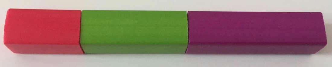
These rods come in all multiples up to 10 of a single unit length, and are colour coded. To keep things simple, we’ve focused only on horizontal composition of rods (interpreted as addition) to form terms, as shown in an example below.

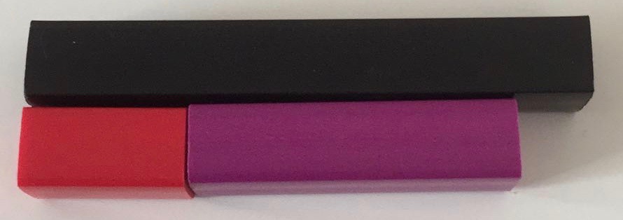
In early primary school, the main relationships being explored relating to horizontal composition are equality and inequality. For example, the figure below shows that black > red + purple, because of the overhanging top-right edge.

With this in mind, we can interpret any such sentence in Cuisenaire rods as an equivalent sentence in (first order) arithmetic. After having done so, we can easily prove mathematically that all such sentences are true. Expressibility and truth coincide for this Cuisenaire syntax! Note that this is very different to the usual abstract syntax for expressing number facts: although 4 = 2 + 1 is false, we can still write it down. This is one reason – we believe – they are so heavily used in early years education: truths are built through play. We only need to know syntactic rules for composition and we can make many interesting number sentences.

From an abstract algebraic perspective, closure and associativity of composition naturally arise, and so long as children are comfortable with conservation of length under translation, commutativity is also apparent. Additive inverses and identity are not so naturally expressed, resulting in an Abelian semigroup structure, which also carries over to our next tool, the bar model.

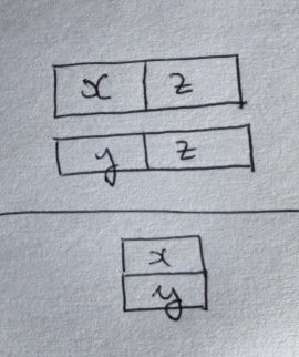
Bar Models

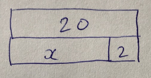
Our investigations suggest that bar models – example for $20 = x+2$ pictured below – are rarely precisely defined in the literature, so one of our tasks was to come up with a precise definition of bar model syntax.

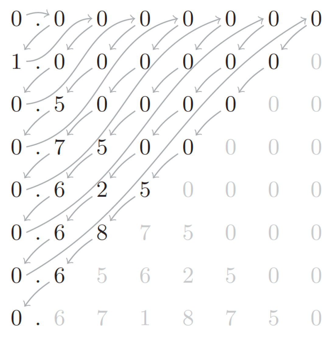
We have made the observation that there seem to be a variety of practices here. The most obvious one, for small numbers drawn on squared paper, is to retain the proportionality of Cuisenaire. These ‘proportional bar models’ (our term) inherit the same expressibility / truth relationship as Cuisenaire structures, of course, but now numerals can exceed 10 – at the cost of decimal numeration being a prerequisite for their use. However, proportionality precludes the presence of ‘unknowns’ – variables – which is where bar models are heavily used in the latter stages of primary schools and in some secondary schools.

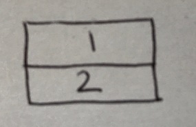
At the other extreme, we could remove the semantic content of bar length, leaving only abutment and the alignment of the right-hand edges as denoting meaning – a type of bar model we refer to as a `topological bar model’. These are very expressive – they correspond to Presburger arithmetic without induction. It now becomes possible to express false statements (e.g. the trivial one below, stating that 1 = 2).

As a result, we must be mathematically precise about valid rules of inference and axiom schemata for this type of model, for example the rule of inference below. Note that due to the inexpressibility of implication in the bar model, many more rules of inference are required than in a standard first-order treatment of arithmetic.

The topological bar model also opens the door to many different mistakes, arising when children apply geometric insight to a topological structure.

In practice, it seems that teachers in the classroom informally use some kind of mid-way point between these two syntaxes, which we call an `order-preserving’ bar model: the aim is for relative sizes of values to be represented, ensuring that larger bars are interpreted as larger numbers. However, this approach is not compositional. Issues arising from this can be seen when trying to model, for example, $x + y = 3$ . The positive integral solutions are either $x = 2, y = 1$ leading to $x > y$ or $x = 1, y =2$ , leading to $y > x$ .

Other Graphical Tools and Manipulatives

As part of our work, we identify certain missing elements from first-order arithmetic in the tools studied to date. It would be great if further work could be done to consider drawings and manipulatives that could help plug these gaps. They include:

Multiplication in bar models. While we can understand $3x$ , for example, as a shorthand for $x + x + x$ , there is no way to express $x^2$
Disjunction and negation. While placing two bar models side-by-side seems like a natural way of expressing conjunction, there is no natural way of expressing disjunction / negation. Perhaps a variation on Pierce’s notation could be of interest?
We can consider variables in a bar model as implicitly existentially quantified. There is no way of expressing universal quantification.
As noted above, these tools capture an Abelian semigroup structure. We’re aware of some manipulatives, such as Algebra Tiles, which aim to also capture additive inverses, though we’ve not explored these in any depth.
We have only discussed one use of Cuisenaire rods – there are many others – as the recent ATM book by Ollerton, Williams and Gregg makes clear, many of which we feel could also benefit from analysis using our approach.
There are also many more manipulatives than Cuisenaire, as Griffiths, Back and Gifford describe in detail in their book, and it would be of great interest to compare and contrast these from a formal perspective.
At this stage, we have avoided introducing a monus into our algebra of bar models, but this is a natural next step when considering the algebraic structure of so-called comparative bar models.
My colleague Dan Ghica alerted me to the computer game DragonBox Algebra 5+, which we can consider as a sophisticated form of virtual manipulative incorporating rules of inference. It would be very interesting to study similar virtual manipulatives in a classroom setting.

An Exciting Starting Point

Charlotte and I hope that attendees at the BSRLM conference – and readers of this blog – are as excited as we are about our idea of the potential for using the tools of mathematical logic and abstract algebra to understand more about early learning of arithmetic. We hope our work will stimulate some others to work with us to develop and broaden this research further.

Acknowledgement

I would like to acknowledge Dan Ghica for reading this blog post from a semanticist’s perspective before it went up, for reminding me about DragonBox, and for pointing out food for further thought. Any errors remain mine.

Know Your Threads

Next week my PhD student Nadesh Ramanathan will present his paper (joint work with Wickerson) on Concurrency-Aware Scheduling for High-Level Synthesis at FCCM 2018.

This work is the latest instalment of our approach to scheduling multithreaded software in high-level synthesis while taking advantage of the weak memory behaviour allowable in the C/C++11 standard.

Our previous work analysed, and then synthesised, each thread individually. What this paper adds is the ability to perform an inter-thread analysis – while still synthesising threads individually. It is natural, in hardware synthesis, to assume knowledge of the other threads that are being synthesised at compile time. We show in this paper that such knowledge can – and often does – considerably improve high-level synthesis results, by removing redundant constraints during the scheduling process.

Readers wanting to know a little more before diving into the paper itself could also read John Wickerson’s description of our work.

FPGA 2018: Some Highlights

The 2018 ACM International Symposium on Field-Programmable Gate Arrays was held at the end of February in its usual venue of Monterey, California. In this post I identify a few of my personal highlights from the conference.

Josipovic, Ghosal and Ienne presented “Dynamically-Scheduled High-Level Synthesis,” a very nice piece of work, which reminded me of my old days with Handel-C from Celoxica, which had at its core a similar dynamic scheduling approach described in Page and Luk’s paper “Compiling Occam into FPGAs” from the first ever FPL conference. One of the several ways Lana’s work goes beyond this is the way it deals with memory accesses, which it disambiguates using a Load Store Queue. I found this interesting – it seems to me that there might be much scope to apply techniques I’ve worked on for the static disambiguation, using both polyhedral methods [1] and separation logic [2], to the problem of generating enough information to produce specialised Load Store Queues for a particular application.

Dai, Liu and Zhang presented “A Scalable Approach to Exact Resource-Constrained Scheduling Based on a Joint SDC and SAT Formulation.” This paper revisited the popular SDC scheduling heuristic of Cong and Zhang and showed how, by combining it with a SAT solver, one can optimally and efficiently solve resource-constrained scheduling problems arising in High-Level Synthesis. Resource constrained scheduling is hard because of the non-convexity in the problem: one may choose to perform operation A before or after operation B when only wanting to use one instance of a resource. It’s this disjunctive constraint that’s heuristically dealt with in the original SDC paper, for which there exist many ILP formulations, and which the authors address with SAT in this paper. I was intrigued by this paper because the learning of SAT conflict clauses done by the tool appeared to me to be very similar in principle to Gomory cuts made by an ILP solver tackling the same problem, and I wondered whether this observation could be made precise and whether it had value the context of the problem at hand.

Mohajer, Wang and Bazargan presented an intriguing paper “Routing Magic: Performing Computations Using Routing Networks and Voting Logic on Unary Encoded Data.” Instead of using a standard positional radix number system, they proposed using a certain form of unary representation under which all digits with the value 1 occur at the start of a word. This allows certain very efficient computations, notably the computation of arbitrary monotonic functions of a single variable, using no logic – only routing. Multi-input functions and non-monotonic functions do require logic, but they showed for some examples that it’s cheaper to have an exponential number of these tiny logic elements than a polynomial number of the larger logic elements that you would get from positional radix number systems. My suspicion is that the scheme would perform particularly poorly on something like a two-input adder, but the authors presented enough examples to convince the audience that there are cases where it performs well. It was an unusual and thought-provoking presentation.

Zheng, Chen, Zhang and Prasanna presented “A Framework for Generating High-Throughput CNN Implementations on FPGAs.” I enjoyed this paper because it explicitly mixed several important things in any good implementation engineering paper: simple analytical models that provide insight into design, good analysis, and lessons that can be reused beyond the case study under consideration, by other designers for other problems.

Congratulations to Kia Bazargan (Programme Chair) for putting together a great programme, and to Jason Anderson (General Chair) for ensuring all the arrangements ran smoothly!

Iterating Exactly

I’m very excited to share that my PhD student, He Li, will tomorrow be presenting his paper ARCHITECT: Arbitrary-precision Constant-hardware Iterative Compute at the IEEE International Conference on Field-Programmable Technology 2017 (joint work also with James Davis and John Wickerson.)

Anyone who has done any numerical computation will sooner or later encounter a loop like this:

while( P(x) ) 
  x = f(x);

Where $P(x)$ denotes a predicate determining when the loop will exit, $f$ is a function transforming the state of the loop at each iteration, and $x$ is – critically – a vector of real numbers. Such examples crop up everywhere, for example the Jacobi method, conjugate gradient, etc.

How do people tend to implement such loops? They approximate them by using a finite precision number system like floating point instead of reals.

OK, let’s say you’ve done your implementation. You run for 1000 iterations and still the loop hasn’t quit. Is that because you need to run for a few more iterations? Or is it because you computed in single precision instead of double precision? (Or double instead of quad, etc.) Do you have to throw away all your computation, go back to the first iteration, and try again in a higher precision? Often we just don’t know.

He’s paper solves this problem. As time progresses, we increase both the iteration and the accuracy to which a given iterate is known, snaking through the two-dimensional iteration / precision space, linearising two countably infinite dimensions into the single countably infinite dimension of time (clock cycle) using a trick due to Cantor.

Screen Shot 2017-12-11 at 13.37.24 — Linearising iteration (vertical) and precision (horizontal) into time (arrows)

This is the essence of our contribution.

To make it work in practice, efficiently in hardware, requires some tricks. For a start, we need to be able to support arbitrary precision arithmetic on finite computational hardware (only memory space growing with precision, not compute hardware). Secondly, we need to compute from most-significant to least-significant digit, iteratively refining our computation as we proceed. This form of computation is not supported naturally by standard binary arithmetic, but is supported by redundant arithmetic. We make use of online arithmetic to enable this transformation.

So now you don’t need to worry – rounding error will not stop you getting your answer. There’s an FPGA design for that.

Passing Data Structures to FPGAs

Next week, my former PhD student and postdoctoral researcher, Felix Winterstein, will present our paper Pass a Pointer: Exploring Shared Virtual Memory Abstractions in OpenCL Tools for FPGAs at the IEEE International Conference on Field-Programmable Technology in Melbourne, Australia.

Before launching his current startup, Xelera, Felix and I worked together on the problem of automating the production of custom memory systems for FPGA-based accelerators. I previously blogged about some highly novel work we’d done during his PhD on high-level synthesis for code manipulating complex data structures like trees and linked lists. Full detail can be found in the book version of his PhD thesis. All this work – as exciting as it is – was based on sequential C code description as the input format to a high-level synthesis tool.

Many readers of this blog will be aware that OpenCL is rapidly becoming viewed as an alternative way to write correctness-portable code for FPGA development, with both Intel and Xilinx offering OpenCL flows based around OpenCL 1.X. However, OpenCL 2.0 offers a number of interesting features around shared virtual memory which could radically simplify programming, at the cost of making the compiler significantly more complex for FPGA-based computation. It is this issue we address in the paper Felix will present next week.

There’s lots of exciting program analysis work that could be built on top of Felix’s framework, and I’m keen to explore this further – if a reader of this blog would like to collaborate in this direction or like to do a PhD in this field, feel free to get in touch.

Perhaps most importantly, Felix’s framework is open source – check it out at https://github.com/constantinides/FPGA-shared-mem and let us know if you use it!

HLS and Power: Some FPL Contributions

This week sees the IEEE International Conference on Field-Programmable Logic and Applications, in Ghent, Belgium. Two of my team are attending to present their research papers on High Level Synthesis and on Run-time Power Estimation. In this post, I briefly summarise the key contributions of these papers.

High-Level Synthesis (HLS) is an important technology, which aims to automatically generate hardware designs from high-level (typically software) descriptions of their behaviour. In a previous blog post, I described some work from my PhD student Junyi Liu (joint with Sam Bayliss) on extending a common paradigm for analysis memory dependences – the polyhedral model – to a parametric version, for efficient pipelining in HLS. This week, Junyi presents an alternative use for the same parametric polyhedral HLS framework: automatic loop tiling (joint work with John Wickerson). Loop tiling is a very common compiler transformation – for example it is often used in matrix-matrix multiplication. The key advantage is to make sure that you only have a small set of data you’re working with at any given moment in time (traditionally for cache, in the FPGA context for embedded scratch-pad memories). The size of this working set can be traded off against the amount of off-chip memory traffic by selection of tile sizes. In a multi-dimensional loop, there are many possible options, and navigating this space is non-trivial. Junyi’s work provides a way to produce an explicit formula for both the memory requirement and the amount of off-chip data traffic required for any given tile size. He can then use nonlinear optimisation techniques to explicitly optimise the traffic subject to any given constraint on buffer size. This work is available as an open-source tool at https://github.com/Junyi-Liu/PolyTSS.

Back in 2016, some work I did with Eddie Hung, James Davis, Josh Levine, Ed Stott and Peter Cheung won the best paper prize at FCCM 2016. We showed that it is possible to use an online (recursive least squares) algorithm to learn the instantaneous power consumption of individual components in an FPGA design, with a view to some kind of run-time manager using this information. The solution worked by monitoring certain signal activity at run-time, but the missing part of the puzzle was which signals to monitor. James’s latest paper, STRIPE, with the same co-authors, answers this question. It turns out that the answer to this problem – as with so many in engineering (and life?) – lies in linear algebra. Golub and Van Loan describe in their classic textbook how QR factorisation can be used to heuristically select a subset of “nearly linearly independent” vectors from a larger set, and it’s this approach that tends to win out when given enough data to work with.