I have just returned from a wonderful trip to California with colleagues and students, into which I managed to pack: visiting AMD for a day of presentations to each other, co-running a workshop on Spatial Machine Learning, attending the ACM FPGA 2024 conference at which my student Martin Langhammer presented, and catching up with international colleagues and with Imperial College alumni and their families. In this blog post I’ll briefly summarise some of the work-related key takeaways from this trip for me.

AMD and Imperial
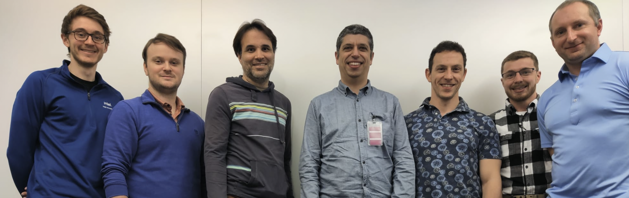
At AMD’s Xilinx campus, I was able to share some of our most recent work. I chose to focus on two aspects: the work we’ve done on e-graphs as an EDA data-structure, and how we have developed these for datapath optimisation, and the development of new highly-efficient LUT-based neural networks. It was great to catch up with AMD on the latest AI Engines developments, especially given the imminent open-sourcing of a complete design flow here. My former PhD students Sam Bayliss and Erwei Wang have been working hard on this – amongst many others, of course – and it was great to get a detailed insight into their work at AMD.
SpatialML Workshop
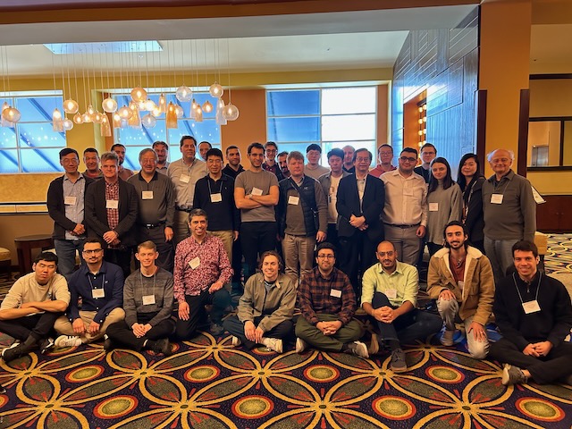
Readers of this blog may know that I currently lead an international centre on spatial machine learning (http://spatialml.net). This year we ran an open workshop, sharing the work we have been doing in the centre, and bringing in additional colleagues from outside the centre too. This was exceptionally well attended: we had delegates from academia and industry internationally in attendance: A*STAR, AMD, Ciena, Cornell, DRW, Essen, Groq, Imperial College, Intel, KAUST, Mangoboost, Minnesota, Rhode Island, Seoul, Simon Fraser, Southampton, Tsinghua, Toronto, and UCLA. We structured the day around a number of excellent academic talks from Zhiru Zhang (Cornell), Vaughn Betz (University of Toronto), Paul Chow (University of Toronto), Lei Xun (University of Southampton), Atefeh Sohrabizadeh (UCLA), and Alex Montgomerie (Imperial College), combined with industrial keynotes from Satnam Singh (Groq) and Sam Bayliss (AMD), closing with a panel discussion on the topic of working across abstraction layers; we had Jason Anderson (U of T), Jason Cong (UCLA), Steve Neuendorffer (AMD) and Wayne Luk (Imperial College) on the panel, with me chairing (sadly Theo Drane from Intel could not make it due to poor weather conditions in Northern California). Slides that are publicly sharable will be made available on the workshop website.
We learned about the use of machine learning (graph representation learning, GNNs) in EDA flows, about scaling LLM implementations across multiple devices in industry and academia, about dynamic DNNs and resource scaling, about programming models and flows for deep learning acceleration in both academia and industry (often using MLIR), and about FPGA architectural enhancements to support more efficient deep learning.
We received very positive feedback from workshop attendees. I would like to express particular thanks to my workshop co-organisers, especially the astoundingly productive Andrew Boutros of the University of Toronto, for all his hard work making this workshop happen.


FPGA 2024
I consider the ACM FPGA conference as my “home” conference: I’m a steering committee member and former chair, but this year my only roles were as a member of the best paper committee and as a session chair, so I could generally sit back and enjoy listening to the high quality talks and interacting with the other delegates. This year Andrew Putnam from Microsoft was technical program chair and Zhiru Zhang from Cornell was general chair. There is of course too much presented in a conference to try to summarise it all, but here are some highlights for me.
- Alireza Khataei and Kia Bazargan had a nice paper, “CompressedLUT: An Open Source Tool for Lossless Compression of Lookup Tables for Function Evaluation and Beyond”, on lossless compression of large lookup tables for function evaluation.
- Ayatallah Elakhras, Andrea Guerrieri, Lana Josipović, and Paolo Ienne have done some great work, “Survival of the Fastest: Enabling More Out-of-Order Execution in Dataflow Circuits”, on enabling (and localising) out-of-order execution in dynamic high-level synthesis, extending the reach of out-of-order execution beyond the approach I took with Jianyi Cheng and John Wickerson.
- Louis-Nöel Pouchet, Emily Tucker and coauthors have developed a specialised approach to checking equivalence of two HLS programs, “Formal Verification of Source-to-Source Transformations for HLS”, for the case where there are no dynamic control decisions (common in today’s HLS code), based on symbolic execution, rewriting, and syntactic equivalence testing. It basically does what KLEE does for corner cases of particular interest to HLS, but much faster. Their paper won the best paper award at FPGA 2024.
- Jiahui Xu and Lana Josipović had a nice paper, “Suppressing Spurious Dynamism of Dataflow Circuits via Latency and Occupancy Balancing”, allowing for a more smooth tradeoff between dynamic and static execution in high-level synthesis than was possible from the early work my PhD student Jianyi Cheng was able to achieve on this topic. They get this through balancing paths for latency and token occupancy in a hardware-efficient way.
- Daniel Gerlinghoff and coauthors had a paper, “Table-Lookup MAC: Scalable Processing of Quantised Neural Networks in FPGA Soft Logic”, building on our LUTNet work and extensions thereof, introducing various approaches to scale down the logic utilisation via sequentialisation over some tensor dimensions and over bits in the linear (LogicNets) case.
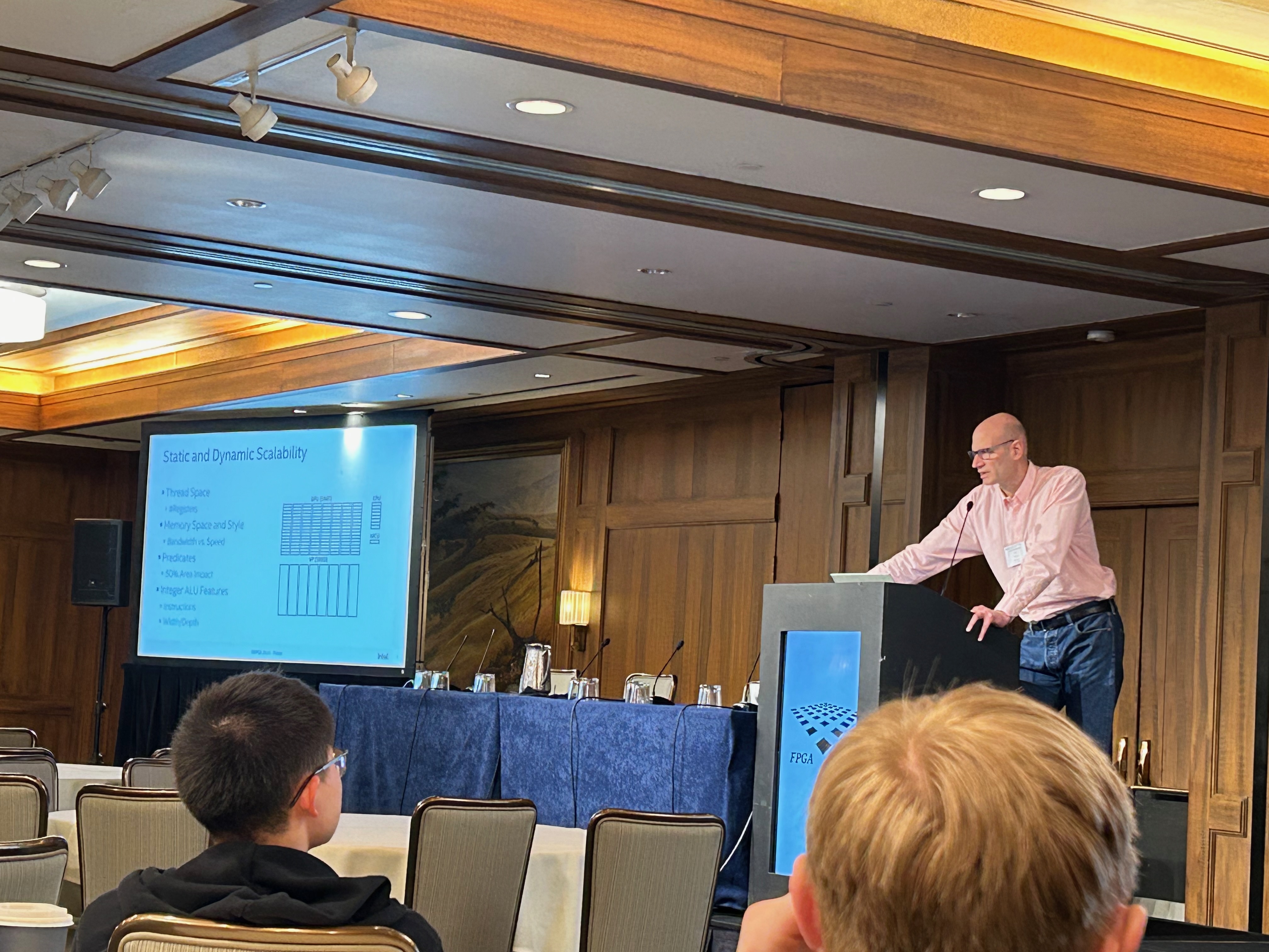
- My PhD student Martin Langhammer (also with Altera) presented his work, “A Statically and Dynamically Scalable Soft GPGPU”, on a super high clock frequency soft GPU for embedding into FPGA designs.
Reflections
I’ve come away with many ideas from all three events: the AMD visit, the workshop, and the FPGA conference. In person attendance at conferences is still the best for this; I didn’t get nearly as many ideas when attending FPGA 2021 or 2022 remotely. It was also particularly satisfying to see our work on soft-logic efficient deep neural networks (starting with LUTNet, most recently PolyLUT) being cited by so many people at the conference; this work appears to have really made a long-term impact.
Finally, it is always a joy to visit Monterey. This year FPGA was held at a hotel on Cannery Row, described by John Steinbeck as “a poem, a stink, a grating noise, a quality of light, a tone, a habit, a nostalgia, a dream”.


 for its inputs
  and some learned weight vector
  and bias
  , where
  is typically a fixed nonlinear function such as a
  . The Xilinx team noted that if they restrict the length of the vector
  . In this way, we can tune a knob: turn down to
  for minimal expressivity but the smallest number of parameters to train, and recover LogicNets as a special case; turn up
 together with
  elements,
  , for
, for  . The numbers represented are (except special values),
  . This is a very flexible starting point, which is to be welcomed, and there is much to explore under this general hood. In all the examples given, the scalar data types are either floating point or integer/fixed point, but there seems to be nothing in the specification specifically barring other representations, which could of course go far beyond traditional block floating point and more recent block exponent biases.
 denotes the
  th element of vector
  ,
,  denotes the scaling of
  (on elements), the (elided) product on scalings and the sum on element products is undefined. The intention, of course, is that we want the dot product to approximate a real dot product, in the sense that
  , where the semantic brackets correspond to interpretation in the base scalar types and arithmetic operations are over the reals. But the nature of approximation is left unstated. Note, in particular, that it is not a form of round-to-nearest defined on MX, as hinted at by the statement “The internal precision of the dot product and order of operations is implementation-defined.” This at least suggests that there’s an assumed implementation of the multi-operand summation via two-input additions executed in some (identical?) internal precision in some defined order, though this is a very specific – and rather restrictive – way of performing multi-operand addition in hardware. There’s nothing wrong with having this undefined, of course, but an MX-compliant dot product would need to have a very clear statement of its approximation properties – perhaps something that can be considered for the standard in due course.
 and
and  are the
  th MX-compliant subvector of
  .” Like in the “Dot” definition, the summation notation is also not defined in the specification, and also this definition doesn’t carry the same wording as for “Dot” on internal precision and order, but I am assuming it is intended to. It is left undefined how to form component subvectors. I am assuming that the authors envisaged the vector
  and
and  are the extracted “close” expressions.
 can just be replaced by
  , e.g.
  . But our original ARITH paper wasn’t able to consider special cases. What we really need for that is some kind of conditional rewrite rules, e.g.
  , where I am using math script to denote the value of a variable and teletype script to denote an expression.
 . Now let’s imagine introducing a new operator
  that takes two expressions, the second of which is interpreted as a Boolean. Let’s give
  . In this way we can ‘lift’ equivalences in a subdomain to equivalences across the whole domain, and use e-graphs without modification to reason about these equivalences. Taking the absolute value example from previously, we can write this equivalence as
  . These
 ![x \in [-1,1]](https://s0.wp.com/latex.php?latex=x+%5Cin+%5B-1%2C1%5D&bg=ffffff&fg=000000&s=0&c=20201002) , then a classical evaluation of
, then a classical evaluation of  would give me
 ![[-2,2]](https://s0.wp.com/latex.php?latex=%5B-2%2C2%5D&bg=ffffff&fg=000000&s=0&c=20201002) , due to the loss of information about the correlation between the left and right-hand sides of the subtraction operator. Once again, our e-graph setting comes to the rescue! Taking this example, a rewrite
, due to the loss of information about the correlation between the left and right-hand sides of the subtraction operator. Once again, our e-graph setting comes to the rescue! Taking this example, a rewrite  would likely fire, resulting in zero residing in the same e-class as
  . Since the interval associated with
  is
is ![[0,0]](https://s0.wp.com/latex.php?latex=%5B0%2C0%5D&bg=ffffff&fg=000000&s=0&c=20201002) , the same interval will automatically be associated with
, the same interval will automatically be associated with 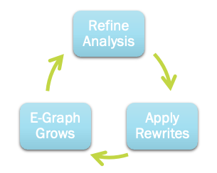

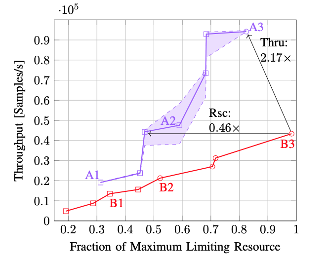
 of ‘hard’ samples I used to characterise the network varies in practice from the actual proportion
  , then I may end up with a somewhat different behaviour, as indicated by the purple region.
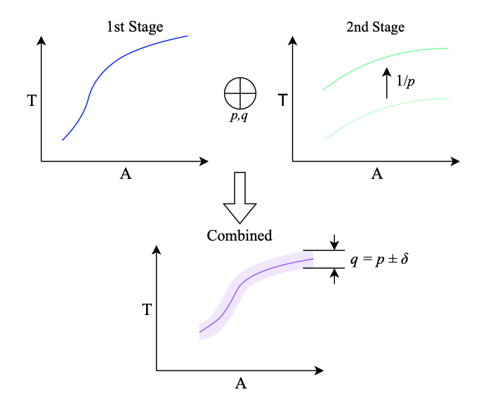

 to denote a function taking two bit vectors and concatenating them together. Of course the ‘multiplication by 10 is easy’ becomes ‘multiplication by 2 is easy’ in binary. Putting this together, we can write
  , meaning that multiplication by two is the same as concatenation with a zero. But what does ‘the same as’ actually mean here? Clearly they are not the same expression syntactically and one is cheap to compute whereas one is expensive. What we mean is that no matter which value of
  rather than
  .
.  then it necessarily follows that
  for every function symbol
  . Like any equivalence relation on a set,
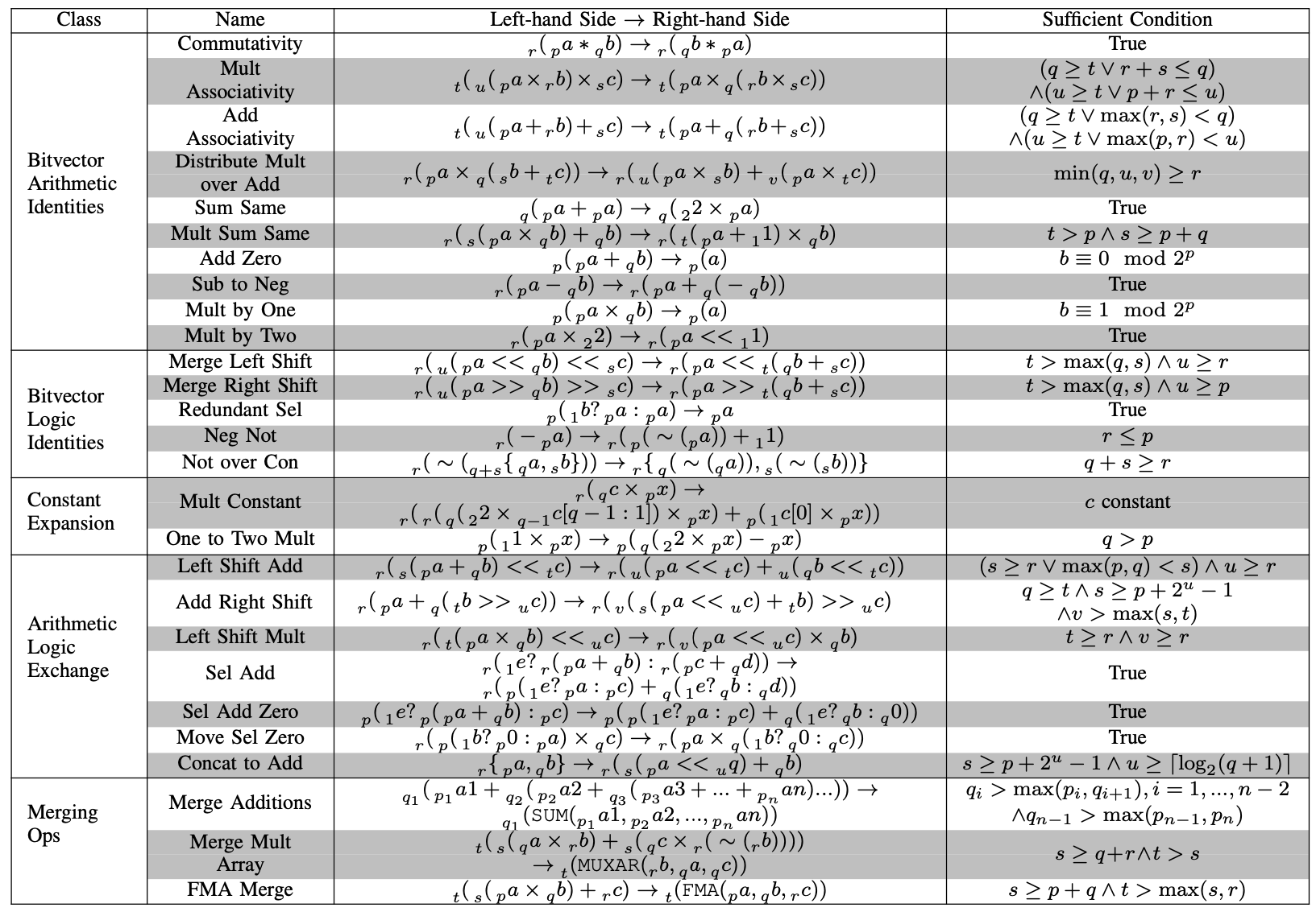
 then I wouldn’t bother to calculate
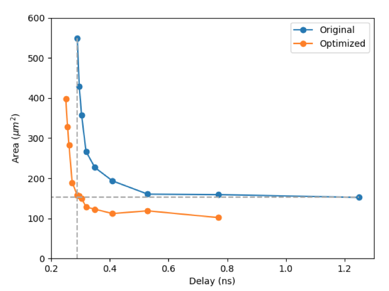
  twice. We describe in our paper how we address this problem via an optimisation formulation. Our tool solves this optimisation and produces synthesisable Verilog code for the resulting circuit.