In my previous post, I argued that block number formats can be understood geometrically as direction preservers. That argument relied on an idealization: once a block direction had been chosen, its scale could be set optimally as an arbitrary real number.
Real hardware formats do not usually work that way. In many practical schemes, block scales are quantized very coarsely, sometimes all the way down to powers of two. In particular, in the MX specification, all the concrete compliant formats use E8M0 scaling.
So does the directional picture I painted in my last post survive this brutal scaling? Here I will argue, in the first of what I hope will be a short sequence of follow-up blog posts, that it does.
From ideal block scales to quantized block scales
Recall the setup from the earlier post. A vector is partitioned into blocks, , and each block is approximated as , where is a low-precision mantissa vector and is a scalar block scale.
In the earlier post, I assumed that was an arbitrary real value, chosen optimally in the least-squares sense. That gave the ideal blockwise representation .
Now let us keep the same mantissa vectors , but suppose that the scale factors themselves must be quantized. Write the implemented scale as , so that the represented block becomes .
It is convenient to define the multiplicative scale error . Then .
Note that, of course, quantizing the block scale does not change the chosen direction of a block at all; it only changes its length. So the only directional distortion comes from the relative rescaling of different blocks.
An exact cosine formula
Let , so that is the fraction of the ideal projected vector’s energy contained in block .
Then it can be shown that (the proof is included at the end of this post).
So the effect of scale quantization on direction depends only on how uneven the factors are across blocks. If all blocks were rescaled by the same factor, direction would be unchanged.
Exponent-only power-of-two scaling
Now consider the coarsest plausible case: each block scale is rounded to the nearest power of two. Then each multiplicative error satisfies .
So, from our exact cosine formula, we are interested in how small can be, when all the lie in the interval .
A simple inequality shows that the answer depends only on the two extreme values of the interval. If all the block rescaling factors lie in , then
(proof at the end of this blog post).
In the power-of-two case we have , , so , and therefore
.
Equivalently, .
So even if every block scale is rounded to the nearest power of two, the resulting vector remains within about of the ideally scaled one.
That is the main result of this post.
One striking feature of the bound is that it does not depend on the dimension of the vector. The reason is that the worst case is already attained by a two-group energy split: some blocks rounded up, others rounded down. Once those two groups exist, adding more blocks or more dimensions does not make the bound worse, as is apparent from the proof below.
20 degrees is less than it sounds
Our everyday intuition may tell us that this angle is not huge, but it’s not that small either. In a sense, that’s true. But angles behave very differently in high-dimensional spaces. In high dimension, most random vectors are almost orthogonal to one another: their angle is close to , so a guarantee that an approximation remains within of the original vector is much stronger than it would sound in two or three dimensions.
Beyond power-of-two
We’ve analysed power-of-two scaling here for two reasons: because it’s in a sense the crudest possible floating-point rounding, and because it’s commonly used in real hardware designs.
That does not mean it’s optimal. But it does raise two further questions. Firstly, we’ve assumed here that the exponent range is sufficiently wide – what if it’s not? Secondly – and relatedly – how much better can this angular bound get by spending some of the scale bits on greater precision?
My view is that the answer becomes clearer once a tensor-wide high-precision scale is introduced, something NVIDIA has recently done. In that setting, the block scales get relieved of their additional duty to capture global magnitude. This will be the subject of the next post on the topic!
Proofs
Readers not interested in the algebra can safely skip this section.
Cosine formula
Recall that for each block .
Then, because the blocks occupy disjoint coordinates, .
Also, , and .
Therefore .
Now, as per the main blog post, define .
Writing , so that , the numerator becomes and the denominator becomes , giving
.
20 degree bound
Assume that all the multiplicative error factors lie in an interval with .
Let .
Then the cosine is just . Since each , we have
.
Expanding this gives
.
Multiplying by and summing over gives
.
Therefore .
Now the weighted mean also lies in the interval , so it remains to minimize
over .
Differentiating shows that the minimum occurs at , the harmonic mean of and .
I’ve recently returned from the SIAM PP 2026 conference and as always, conferences help provide time for research reflection. One thing I’ve been reflecting on during my journey back is the various explanations people give for why the machine learning world is so keen on block number formats (MX, NVFP, etc.) – see my earlier blog post on MX if you need a primer. Many hardware engineers tend to answer that they lead to efficient storage, or efficient arithmetic, or improved data transfer bandwidth, which are all true. But I think there’s another complementary answer that’s less well discussed (if indeed it is discussed at all). I hope this blog post might help stimulate some discussion of this complementary take.
On the numerical side, at first glance it might seem surprising that despite these formats representing numbers with very limited precision, large neural networks often tolerate them remarkably well, with little loss in accuracy. In my experience, most explanations focus on dynamic range, quantization noise, the inherent noise robustness of neural networks, or calibration techniques. But I suspect there is also a simple geometric way to think about what these formats are doing: Block number formats help preserve vector direction. And for many machine learning computations, preserving direction matters far more than preserving exact numerical values.
Block formats inherently represent direction and magnitude
Consider a vector whose coordinates are partitioned into blocks .
In a block format, each block is represented using a shared scale and low-precision mantissas. For ease of discussion, we’ll consider the simplest case here, where scales are allowed to be arbitrary real-valued. In general, they may be much more restricted, e.g. powers of two.
Each block is approximated as
where
is a vector of low-precision mantissas, and
is a scalar shared scaling factor.
In other words, each block can be thought of as a direction (encoded by the mantissas) multiplied by a magnitude (the shared scale). Strictly speaking, the mantissa vectors need not be normalized, and in many formats their entries may have quite different magnitudes (for example in integer mantissa formats such as MXINT). However this does not change the geometry. The representation is invariant to rescaling of : multiplying by any constant simply rescales by the inverse factor. What matters for the approximation is therefore only the direction of , i.e. the one-dimensional subspace it spans.
Often we don’t think of it like this, but broadly speaking this is what has happened: block scaling allows us to decouple magnitude and direction representation. This resembles the familiar decomposition of a vector into its magnitude and direction, but applied locally within blocks.
If the mantissa vector points roughly in the same direction as the original block , then scaling it appropriately produces a good approximation of that block.
OK, but does preserving directions block by block actually preserve the direction of the whole vector? It turns out that the answer is yes.
Direction Preservation
Let us make the reasonable assumption that the scale of each block is not chosen arbitrarily, but rather is the best possible scale for that block in the least squares sense, for whatever mantissa vector we choose, i.e. . Then is the orthogonal projection of onto the line spanned by .
So to what extent do the approximate and the original block vector point in the same direction? We can measure the block cosine similarities of the blocks as: .
Equally, we can measure the the cosine similarity of the full vectors (the concatenation of the original blocks versus the concatenation of the approximated blocks): .
My aim here is to explain why small error in direction at block level leads to small error at vector level.
First, let’s define , which we can think of as the fraction of the vector’s energy contained in block ; these add to 1 over the whole vector. Now we can state the result:
Theorem (Block Cosines)
Under the blockwise least-squares scaling, .
For proof, see end of post.
In simple terms, this theorem states that the cosine similarity of the whole vector is the energy-weighted RMS of the block cosine similarities.
What are the implications?
The weights represent how much of the vector’s energy lies in each block. Blocks that contain very little energy contribute very little to the final direction. The important consequence is that direction errors do not accumulate catastrophically across blocks. Instead, the overall directional error simply depends on a weighted average of the block direction errors. In other words, if block number formats preserve the directions of individual blocks, they automatically preserve the direction of the entire vector.
Many core operations in machine learning depend heavily on vector direction. Notably, during training, stochastic gradient descent updates are already in the form of magnitude (learning rate) + direction. We already have a knob controlling magnitude (the learning rate); what matters is that the direction is preserved. In attention mechanisms and embedding, directional similarity measures are very important. Even for the humble dot product, the workhorse of inference, preservation of direction means that small perturbations in input give rise to only small perturbations in output, so the dot product behaves robustly.
Conclusion
Block floating-point and similar formats like block mini-float, MX, NVFP, are usually explained in terms of dynamic range and quantization noise. But geometrically, I like the perspective that they do something simpler: they approximate each block of a vector as direction × magnitude.
And as long as the block directions are preserved reasonably well, the direction of the whole vector is preserved too.
I think this is a useful intuition as to why very low-precision formats can work so well in modern machine learning systems. Block number formats are, in a very real sense, direction preservers. From this perspective, such low-precision block formats succeed not because they represent individual numbers accurately, but because they preserve the geometry of vectors.
Lots of extensions of this kind of analysis are of course possible. To name just a few:
We’ve focused on vectors, but tensor-level scaling may have interesting interplay with batching during training, for example
We made the simplifying assumption that scaling factors were real valued, but these can be restricted, most significantly to powers of two, and the analysis would need to be modified to incorporate that change.
We’ve not discussed mantissas at all, lots more of interest could be said here.
Potentially this approach could help provide some guidance to the empirical sizing of blocks in a block representation.
If anyone would like to work with me on this topic, do let me know your ideas.
Proof of the theorem
Readers not interested in the algebra can safely skip this section.
For each block , the approximation with chosen by least squares is the orthogonal projection of onto the line spanned by .
So we can write where is orthogonal to .
Taking the inner product with gives .
Now sum over blocks. Because the blocks correspond to disjoint coordinates,
This month I took a trip to California for the FPGA 2026 conference, together with my two new PhD students Ben Zhang and Bardia Zadeh, which I combined with a number of visits in the San Francisco Bay Area in the days preceding the conference. This post provides a brief summary of my visit.
First up on our travels was dinner with Rocco Salvia. Rocco was my Research Assistant – we worked together some years ago on automating the analysis of average-case numerical behaviour of reduced-precision floating-point computation. He is now working for Zoox, the robotaxi company owned by Amazon where his first-rate engineering skills are being put to good use!
The following day we went to visit Max Willsey at UC Berkeley and his PhD student Russel Arbore. Max and I (together with others) organised a Dagstuhl workshop on e-graphs recently, and we went to pick up the research conversations we left behind a month ago in Germany and spend some good quality whiteboard time together. Russel and Max are working on some really exciting problems in program analysis.
That afternoon, we had the chance to catch up with my old friend and colleague Satnam Singh, now working for the startup harmonic.fun. Harmonic is a really exciting company, combining modern AI tools with Lean-based formal theorem proving. Expect great things here.
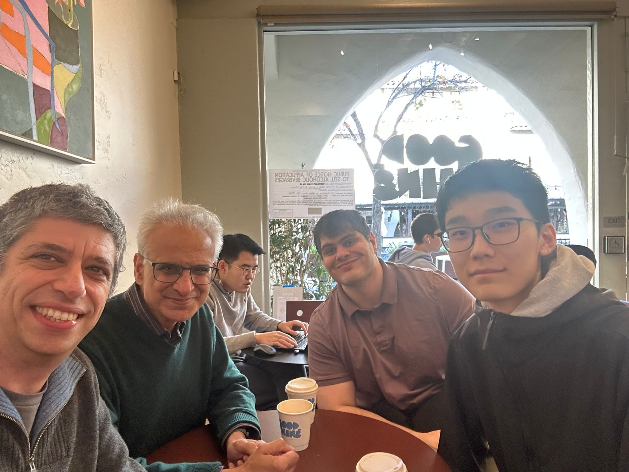
George, Satnam, Bardia and Ben, enjoying coffee near the Harmonic office.
The following morning, we went to visit AMD, with whom I have longstanding collaborations. Amongst others, we met my two former PhD students Sam Bayliss and Erwei Wang there, and discussed our ongoing work on e-graphs and on efficient machine learning, as well as finding out the latest work in Sam’s team at AMD including their release of Triton-XDNA.
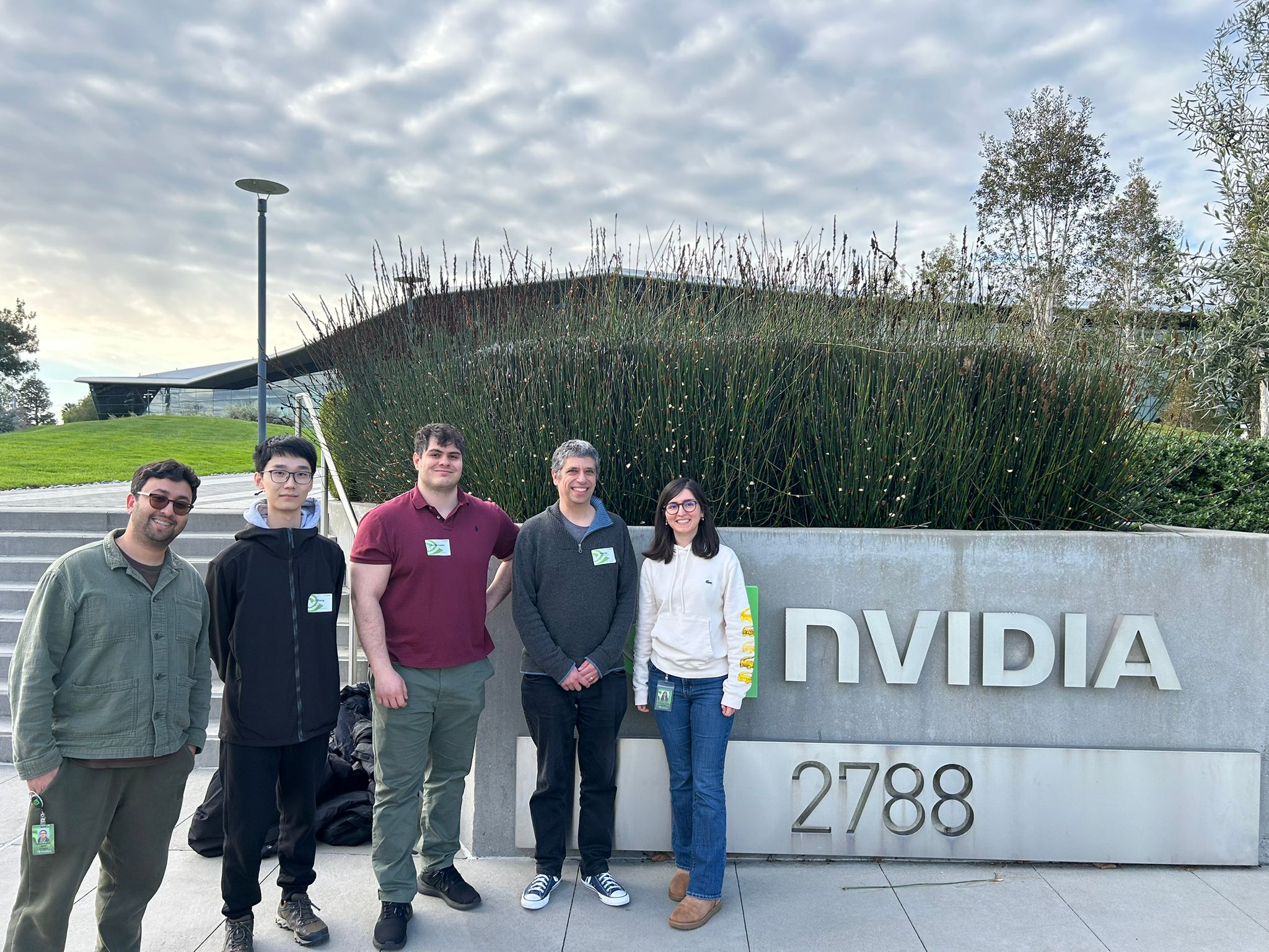
Rajarshi, Ben, Bardia, George and Atefeh at NVIDIA
It has long been a tradition that Peter Cheung, when in the Bay Area, organises a get-together of alumni of the Circuits and Systems Group (formerly Information Engineering group, when Bob Spence was Head of Group). This time was no exception – we met up with many of our department’s former students, and some came to a great dinner too. It’s always a delight to hear about the activity of our alumni, spread across the tech companies in the Bay Area.
CAS group Bay Area alumni dinner
After a flying visit to my former PhD student’s family, we then made it down to Monterey for FPGA 2026. Regular readers of this blog will know that I’ve been attending FPGA for more than 20 years, have been Program Chair, General Chair, Finance Chair and am now Steering Committee member of the conference. So it always feels a little like “coming home”. I also love Monterey – despite the touristy bits – and am a fan of Steinbeck‘s writing in which he immortalised Monterey with some of the best opening lines ever (of Cannery Row): “Cannery Row in Monterey in California is a poem, a stink, a grating noise, a quality of light, a habit, a nostalgia, a dream.”
This year, the general chair of FPGA 2026 was Jing Li, and the great programme was put together by Grace Zgheib.
My favourite paper at FPGA this year also won the best paper prize. Duc Hoang and colleagues identified that Kolmogorov-Arnold Networks are a natural fit to the LUT-based neural networks my group pioneered e.g. [1,2]. They form a really interesting design point, overcoming the exponential scaling of area with the product of precision and neuron fanin present in both my SOTA work with Marta Andronic and earlier work like Xilinx LogicNets, to produce a design that scales exponentially only in the precision. I very much enjoyed reading this paper and seeing it presented, and I think it opens up new areas of future work in this area.
Duc Hoang and his coauthor Aarush Gupta, receiving the best paper award from Grace and Jing
I also particularly enjoyed the work of Shun Katsumi, Emmet Murphy and Lana Josipović (ETH Zurich) on eager execution in elastic circuits. I previously collaborated with Lana on elastic circuits, and it’s great to see the latest work in this area and the use of formal verification tools to prove correctness of performance enhancements. I had a very nice discussion with Lana about possible ways to take this work further.
Rouzbeh Pirayadi, Ayatallah Elakhras, Mirjana Stojilović and Paolo Ienne (EPFL) had a really interesting paper on avoiding the overhead of load-store queues in dynamic high-level synthesis. (This paper was also the runner-up best paper).
From my own institution, Oliver Cosgrove, Ally Donaldson and John Wickerson had a great paper on fuzzing FPGA place and route tools, which has led a vendor to fix a bug they uncovered through their tool.
There were many other good papers, but just to mention a couple that I found particularly aligned to my own interests: EdgeSort on the design of line-rate streaming sorters and HACE on extracting CDFGs from RTL were both really interesting to hear presented.
It was great to be reunited with so many international colleagues and to provide my new students Bardia and Ben with the chance to begin their journey of integration into this welcoming community.
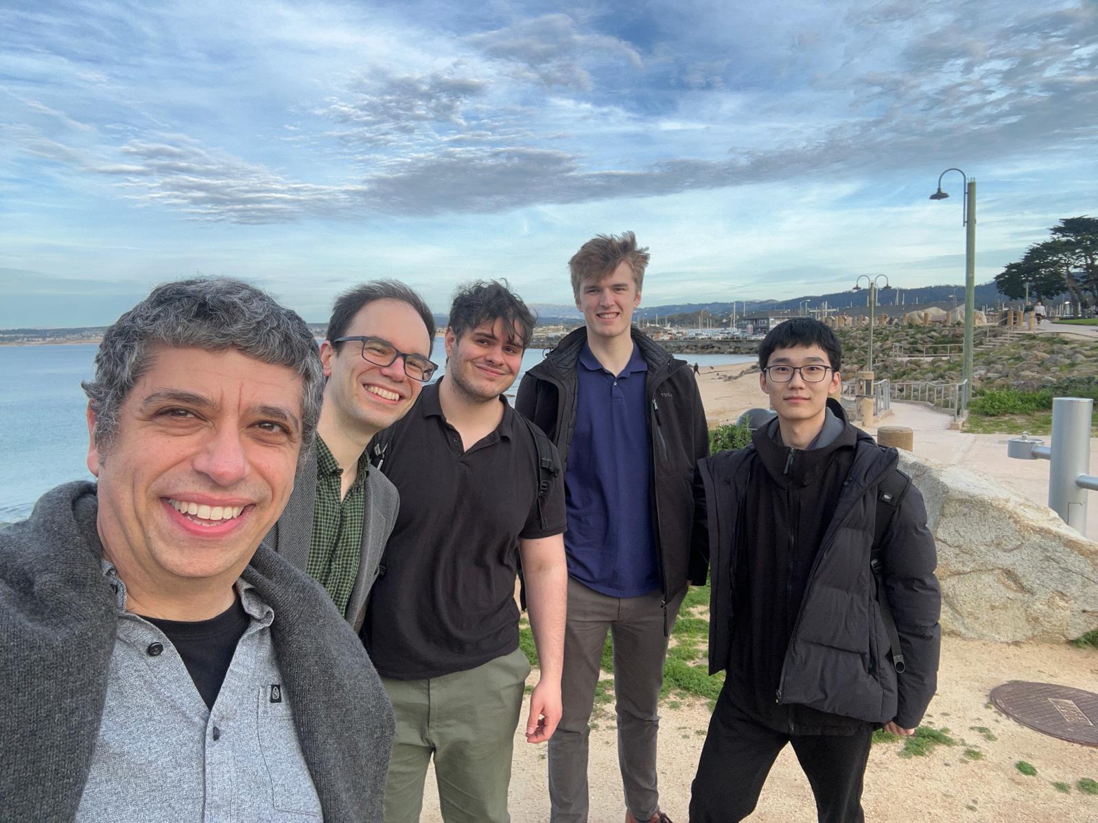
Me, John, Bardia, Oliver and Ben after the end of the final conference session
I’ve always struggled with the concept of “doing your best”, especially with regards to avoiding harm. This morning from my sick bed I’ve been playing around with how I could think about formalising this question (I always find formalisation helps understanding). I have not got very far with the formalisation itself, but here are some brief notes that I think could be picked up and developed later for formalisation. Perhaps others have already done so, and if so I would be grateful for pointers to summary literature in this space.
The context in which this arises, I think, is what does it mean to be responsible for something, or even to blame? We might try to answer this by appeal to social norms: what the “reasonable person” would have done. But in truth I’m not a big fan of social norms: they may be politically or socially biased, I’m never confident that they are not arbitrary, and they are often opaque to those who think differently.
So rather than starting from norms, in common with many neurodivergents, I want to think from first principles. How should we define our own responsibilities when we act with incomplete information? And what does it mean to be “trying one’s best” in that situation? And how do we not get completely overwhelmed in the process?
Responsibility and Causality
One natural starting point is causal responsibility. If I take action A and outcome B occurs, we ask: would B have been different if I had acted otherwise? Causal models could potentially make this precise through counterfactuals. This captures the basic sense of control: how pivotal was my action?
But responsibility isn’t just about causality. It is also about what I knew (or should have known) when I acted.
Mens Rea in the Information Age
The legal tradition of mens rea, the “guilty mind”, is helpful here. It recognises degrees of responsibility, such as:
Intention: I aimed at the outcome.
Knowledge: I knew the outcome was very likely.
Recklessness: I recognised a real risk but went ahead regardless.
Negligence: I failed to take reasonable steps that would have revealed the risk.
It’s the final one of these, negligence, that causes me the most difficulty on an emotional level. A generation ago, a “reasonable step” might be to ask a professional. But in the age of abundant online information, the challenge is defining what “reasonable steps” now are. No one can read everything, and I personally find it very hard to draw the line.
If we had knowledge of how the information we gain increases with the time we spend collecting that information, we would be in an informed place. We could decide, based on the limited time we have, how long we wish to explore any given problem.
From Omniscient Optimisation to Procedural Reasonableness
However, we must accept that there are at least two levels of epistemic uncertainty here. We don’t know everything there is to know, but nor do we even know how the amount of useful information we collect will vary based on the amount of time we put in. Maybe just one more Google search or just one more interaction with ChatGPT will provide the answer to our problem.
In response, I think we must shift the benchmark. Trying one’s best does not mean picking the action that hindsight reveals as correct. It means following a reasonable procedure given bounded time and attention.
So what would a reasonable procedure look like? I would suggest that we start with the most salient, socially-accepted, and low-cost information sources. We then keep going with our investigation until further investigation is unlikely to change the decision in proportion to its cost.
In principle, we may want to continue searching until the expected value of more information is less than its cost. But of course, in practice we cannot compute this expectation.
A workable heuristic appears then to be to allocate an initial time budget for exploration, and if by the end the information picture has stabilised (no new surprises, consistent signals), then stop and decide.
I suspect there is a good Bayesian interpretation of this heuristic.
The Value of Social Norms
What then of social norms? What counts as an obvious source, an expert, or standard practice, is socially determined. Even if I am suspicious of social norms, I have to admit that they carry indirect value: they embody social learning from others’ past mistakes. Especially in contexts where catastrophic harms have occurred such as in medicine and engineering, norms, heuristics and rules of thumb represent distilled experience.
So while norms need (should?) not be obeyed blindly, they deserve to be treated as informative priors: they tell us about where risks may lie and which avenues to prioritise for exploration.
Trying One’s Best: A Practical Recipe
Pulling these threads together, perhaps “trying one’s best” under uncertainty means:
Start with a first-principles orientation: aim for causal clarity and avoid blind conformity.
Consult obvious sources of information and relevant social norms as informative signals.
Allocate an initial finite time for self-investigation.
Stop when information appears stable. If significant new evidence arises during investigation, continue. The significance threshold should vary depending on the potential impact.
Document your reasoning if you depart from norms.
Responsibility is not about hindsight-optimal outcomes. It is about following a bounded, transparent, and risk-sensitive procedure. Social norms play a role not as absolute dictates, but as evidence of collective learning obtained in the context of a particular social environment. Above all, “trying one’s best” means replacing the impossible ideal of omniscience with procedural reasonableness.
While this approach still seems very vague, it has at least helped me to put decision making in some perspective.
Acknowledgements
The idea for this post came as a result of discussions with CM over the last two years. The fleshing out of the structure of the post and argument were over a series of conversations with ChatGPT 5 on 26th October 2025. The text was largely written by me.
This blog post sets up and analyses a simple mathematical model of Marx’s controversial “Law of the Tendency of the Rate of Profit to Fall” (CapitalIII §13-15). We will work under a simple normalisation of value that directly corresponds to the assumption of a fixed labour pool combined with the labour theory of value (LTV). I will make no remarks on the validity of LTV in this post, but all results are predicated on this assumption. We will also work in the simplest possible world of two firms, each generating baskets containing both means of production and consumer goods, and in which labour productivity equally improves productivity in the production of both types of goods. I will provide the mathematical derivations in sufficient detail that a sceptical reader can reproduce them quite easily with pen and paper.
The key interesting results I am able to derive here are:
If constant capital grows without bound, then the rate of profit falls, independently of any assumption on the rate of surplus value (a.k.a. the rate of exploitation).
There is a critical value of productivity (which we derive), above which innovation across firms raises the rate of profit of both firms, and below which the rate of profit is reduced.
There are investments that could be made by a single firm to raise its own productivity high enough to improve its own rate of profit when the competing firm does not change its production process. (We locate this threshold, ). However, none of these investments would reduce the rate of profit of when rolled out across both firms (i.e. ). There is therefore no “prisoner’s dilemma” of rates of profit causing capital investment to ratchet up.
However, a firm motivated by increasing its mass of profit (equivalently, its share of overall surplus value) is motivated to invest in productivity above a third threshold , which we also prove exists, and show that . Thus there is a range of investments that improve the profit mass of a single firm but also reduce the rate of profit when rolled out to both firms.
As a result, under the assumptions with which I am working, we can interpret Marx’s Law of the Tendency of the Rate of Profit to Fall to be an accurate summary of economic evolution in purely value terms, under the assumption that firms often seek out moderately productivity-enhancing innovations, so long as radically productivity-enhancing innovations are rare.
1. The Law of the Tendency of the Rate of Profit to Fall
Marx famously argued that the very innovations that make labour more productive eventually pull the average rate of profit downward. My understanding as a non-economist is that, even in Marxian economic circles, this law is controversial. Over my summer holiday, I have been reading a little about this (the literature is vast) and there are many complex arguments on both sides, often very wordy or apparently relying on assumptions that do not line up with a simple LTV analysis.
The aim of this post is thus to show, in the simplest possible algebra, how perfectly reasonable investment decisions by competitive firms reproduce Marx’s claim, providing explicit analysis for how the scale of productivity gains impact on the rate of profit and on individual motivating factors for the firms involved.
2. Set-up and notation
I will be working purely in terms of value, as I understand it from Capital Volume 1, i.e. socially necessary labour time (SNLT) – I will pass a very brief comment on price at the end of the post. We will use the following variables throughout the analysis, each with units of “socially necessary labour time per unit production period”.
Symbol
Definition
Economic reading in Capital
overall constant capital
machinery + materials
overall variable capital
value of wages
overall surplus value
unpaid labour
constant capital advanced by Firm i
machinery + materials
variable capital advanced by Firm i
value of wages
In addition, we will consider the following dimensionless scalar variables:
Symbol
Definition
Economic reading in Capital
The baseline production rate of commodities by Firm 2, as a multiple of that produced by Firm 1
capital deepening factor: the ratio of the post-investment capital advanced to the pre-investment capital advanced, evaluated in terms of SNLT at the time of investment
dearer machine (III §13)
labour-productivity factor: the ratio of the number of production units produced per unit production time post-investment to the same quantity prior to the investment.
fewer hours per unit (III §13)
We will work throughout under the constraint that . This can be interpreted as Marx’s “limits of the working day” (CapitalI §7) and flows directly from the LTV. Below I will refer to this as “the working day constraint”.
Before embarking on an analysis of productivity raising, it is worth understanding the rate of profit at an aggregate level. Marx defined the rate of profit as:
During my reading on the rate of profit, I have seen a number of authors describe the tendency of the rate to fall in the following terms: divide numerator and denominator by , to obtain . At that point an argument is sometimes made that keeping (the rate of surplus labour, or the rate of exploitation) constant (or bounded from above), as as . This immediately raises two questions: why should remain constant (or bounded), and why should ? In this post, I will attempt to show that the first of these assumptions is irrelevant, while providing a reasonable basis to understand the second. As a prelude, we will now prove the following elementary theorem:
Theorem 1 (Rate of Profit Declines with Increasing Capital Value). Under the working-time constraint, .
Proof.. □
It is worth noting that implies that , but the latter is not sufficient for – a simple counterexample would be to keep constant while , leading to an asymptotic rate of profit of .
Theorem 1 forms our motivation to consider why we may see increasing without bound. To understand this, we will be considering three scenarios:
Scenario A: the baseline. Each firm is producing in the same way, but they may have a different scale of production. We will normalise production of Firm 1 to 1 unit of production, with Firm 2 producing units of production per unit production time.
Scenario B: after a general rise in productivity. Each firm is again producing in the same way, with the same ratio of production units as Scenario A. Each firm has, however, made the same productivity-enhancing capital investment, so that Firm 1 is now producing units and Firm 2 is now producing units of production per unit time.
Scenario C: only a single firm, Firm 1, implements the productivity-enhancing capital investment. Firm 1 is now producing units and Firm 2 is still producing units of production per unit time. This scenario allows us to explore differences in rate and mass of profit for Firm 1 compared to Scenario A and Scenario B, proving several of the results mentioned at the outset of this post.
3. Scenario A — baseline
We have: and .
The total value of the units of production produced is (using the working day constraint). Each unit of production therefore has a value of . Firm 1 is producing 1 of these units.
The surplus value captured by (profit mass of) Firm 1 is therefore .
This gives an overall rate of profit for Firm 1 of: .
This rate of profit is the same for Firm 2, and indeed for the overall combination of the two. We now have a baseline rate and mass of profit, against which we will make several comparisons in the next two scenarios.
4 Scenario B — both firms upgrade
In this scenario, both firms upgrade their means of production, leading to productivity boost by a factor of , after an increase in the value of capital advanced by a factor of . We will assume that the firms keep the number of working hours constant, and ‘recycle’ the productivity enhancement to produce more goods rather than to drop the labour time employed.
We must carefully consider the impact on the value of variable and fixed capital of this enhancement. The value of variable capital has decreased by a factor , because it is now possible to meet the same consumption needs of the workforce with this reduced SNLT. Of course, we could make other assumptions, e.g. the ability of the labour force to ‘track’ productivity gains in terms of take-home pay, but the assumption of fixed real wages appears to be the most conservative reasonable assumption when it comes to demonstrating the fall of the rate of profit. Equally, the value of the fixed capital has reduced from the original for Firm to , because a greater investment has been made at old SNLT levels () but this investment has itself depreciated in value due to productivity gains. Marx refers to this as ‘cheapening’ in Capital III §14.
We will use singly-primed variables to denote the quantities in Scenario B, in order to distinguish them from Scenario A. We have:
The total value of the units of production produced is . Remembering that our firms together now produce units of production, each unit therefore has value .
Firm 1 is responsible for of these units, and therefore a value of . We may therefore calculate the portion of surplus labour it captures as:
, and its rate of profit as:
.
Simplifying, we have
.
These will be the same rate for Firm 2 (and overall) and a proportionately scaled mass for Firm 2.
It is clear that , i.e. profit mass is always increased by universally adopting an increased productivity (remember we are keeping real wages constant). However, it is not immediately clear what happens to profit rate.
Theorem 2 (Critical productivity rate for universal adoption). For any given set of variables from Scenario A, there exists a critical productivity rate . We have iff .
Proof. Firstly, we will establish that . This follows from the fact that and are both strictly less than 1.
Now iff . Clearing (positive) denominators and noting gives the equivalent inequality . Isolating gives . □
The the overall rate of profit in Scenario 2 can rise or fall, depending on the level of productivity those gains bring. The more the cost of the new means of production, the less is spent on wages, and the greater the fixed-capital intensive nature of the production process, the higher the productivity gain required to reach a rise in profit rate, arguably raising the critical threshold as capitalism develops. However, the fact that and that indicates it will always raise the rate of profit to invest in a productivity gain that’s more than the markup in capital required to implement that gain. That it is still beneficial for the overall rate of profit to adopt productivity gains less significant than the markup in capital expenditure, i.e. when , appears to be consistent with Marx’s Capital III §14, where he appears to be assuming this scenario.
5 Scenario C — Firm 1 upgrades alone
We are interested in now exploring a third scenario: the case where Firm 1 implements a way to increase its own productivity through fixed capital investment, but this approach is kept private to Firm 1. This scenario is useful for understanding cases that may motivate Firm 1 to improve productivity and to understand to what degree they differ from the cases motivating both firms to improve productivity by the same approach.
As per Scenario B, it is important to understand the changes to the SNLT required in production. In Capital I §1, it is clear that Marx saw this as an average. A suitable cheapening factor for labour in these circumstances is because with the same labour () as in Scenario A, we have gone from the overall social production of units of production ( from Firm 2 and 1 from Firm 1), to units of production.
In this scenario we will use doubly primed variable names to distinguish the variables from the former two scenarios. We will begin, as before, with fixed capital, noting that both firms’ capital and labour has cheapened through the change in SNLT brought about by the investment of Firm 1, however Firm 1 also bears the cost of that investment:
and .
.
The total value of the units of production produced by both firms during unit production time is now .
This means that since units of production are being produced, each unit of production now has value . As we did for Scenario B, we can now compute the value of the output of production of Firm 1 by scaling this quantity by , obtaining output value . We may then calculate the surplus value captured by Firm 1 by subtracting the corresponding fixed and variable capital quantities, remembering that both have been cheapened by the reduction in SNLT:
.
The first term in this profit mass expression simply reveals the revalued living labour contributed. The second term is intriguing. Why is there a term that depends on fixed capital value when considering the profit mass under the labour theory of value? Under the assumptions we have made, this happens because although fixed-capital-value-in = fixed-capital-value-out at the economy level, this is no longer true at the firm level; this corresponds to a repartition of SNLT in the market between Firm 1 and Firm 2, arising due to the fundamental assumption that each basket of production has the same value, independently of how it has been made. It is interesting to note that this second term, corresponding to revalued capital, changes sign depending on the relative magnitude of and . For , the productivity gain is high enough that Firm 1 is able to (also) boost its profit mass by capturing more SNLT embodied in the fixed capital, otherwise the expenditure will be a drag on profit mass, as is to be expected.
Now we have an explicit expression for , we may identify the circumstances under which profit mass rises when moving from Scenario A to Scenario C.
Theorem 3 (Critical Productivity Rate for Solo-Profit Mass Increase). For any given set of variables from Scenario A, there exists a critical productivity rate for which we have iff .
Proof. We will begin by considering the difference between surplus value captured in Scenario C and that captured in the baseline Scenario A. We will consider this as a function of .
.
Differentiating with respect to ,
.
Both denominators are positive. The first numerator is clearly positive. The second numerator is also positive for . Hence is strictly increasing over the interval .
Now note that as , . However, at , simplifies to . Hence by the intermediate value theorem and strict monotonicity there is a unique value with such that iff . □
At this point, it is worth understanding where this critical profit-mass inducing productivity increase lies, compared to the value we computed earlier as the minimum required productivity increase in Scenario B required to improve the rate of profit. It turns out that this depends on the various parameters of the problem. However, a limiting argument shows that for large Firm 1, any productivity enhancement will improve profit mass, whereas for small Firm 1 under sufficiently fixed-capital-intensive production, only productivity enhancements outstripping capital deepening would be sufficient:
Theorem 4 (Limiting Firm Size and Solo-Profit Mass). As , . As , .
Proof. Both statements follow by direct substitution into the expression for given in the proof of Theorem 3 and taking limits. □
It is worth dwelling briefly on why there is this dichotomous behaviour between large and small firms. A large Firm 1 () has an output that dominates the value of the product; it takes the lion share of SNLT, and the only impact on the firm of raising its productivity is to reduce the value of labour power as measured in SNLT, which will always be good for the firm. However, a small Firm 1 () has no impact on the value of the product or of labour power. It is certainly able to recover more overall value from the products in the market (the term ), but it must carefully consider its outlay on fixed-capital. In particular if , only small – a low capital intensity – would lead to a rise in profit mass.
So at least for large firms (or low capital intensity) there is a range of productivity enhancements that will induce a rise in profit mass for solo adopters (Scenario C) but would lead to a fall in the overall rate of profit when universally adopted (Scenario B).
It is now appropriate to consider the individual rate of profit of Firm 1 in Scenario C, having so far concentrated only on the mass of profit.
The rate of profit of Firm 1 in Scenario C is:
.
As with the mass of profit, we are able to demonstrate the existence of a critical value of productivity, above which Firm 1 increases its rate of profit as a solo adopter:
Theorem 5 (Critical Productivity Rate for Solo-Profit Rate Increase). For any given set of variables from Scenario A, there exists a critical productivity rate for which we have iff .
Proof. As per the proof of the profit mass case, we will firstly compute the difference between the two scenarios, which we will denote . Forming a common denominator that does not depend on between the expressions for and allows us to write where . Note that is differentiable for , with:
Hence is strictly increasing with .
Now let’s examine the sign of as . Firstly, by direct substitution, , where we have also recognised that , total surplus value in Scenario A, is . This expression simplifies to . Of the three multiplicative terms, the first is negative () while the other two are positive. Hence becomes negative as , and hence so does .
We should also examine the sign of at . This time, , which simplifies to . Since both multiplicative terms are positive, and hence is positive.
So again we can make use of the intermediate value theorem, combined with our proof that is strictly increasing to conclude that there exists a unique such that iff , completing the proof. We have already shown that that via the second half of the sign-change argument. □
It remains, now, to try to place in magnitude compared to the other critical value we discovered, :
Theorem 6 (Productivity required for solo rate improvement dominates that required for universal rate improvement)..
Proof. We can place our earlier expressions for and over a common denominator that does not depend on . Here and where and .
Note that . Evaluating at , we have . From Theorem 2, we know that and so the second term is negative and so .
Since was independent of and positive, we can conclude that . However, we also know that by definition of . Hence . And we may therefore conclude that . □
This theorem demonstrates that there is no “prisoner’s dilemma” when it comes to rate of profit in this model: if a firm is motivated to invest in order to raise its own rate of profit ( then that investment will also raise overall rate of profit if implemented universally.
6. Summary of Thresholds
We have demonstrated a number of critical thresholds of productivity increase. Collecting results, we have
In the case of large firms (or production that is sufficiently low in fixed-capital input), we may also write:
A numerical example of these thresholds is illustrated below, for the large firm case.
Several conclusions flow from this order:
There are no circumstances under which a firm, to improve its rate of profit, makes an investment that will not also improve the rate of profit if universally adopted ().
There are cases, especially for large firms, where investments that may be attractive from the perspective of improving profit mass nevertheless reduce profit rate ().
There are productivity-enhancing investments that may be unattractive from a purely driven (either mass or rate).
7. Conclusion: The Falling Rate of Profit
In this model, we can conclude that continuous investment in moderately productivity-enhancing means of production () will lead to a falling rate of profit. Overall capital value will grow, which (Theorem 1) will lead to a falling rate of profit independent of assumptions on the rate of exploitation (rate of surplus value) .
The results in this post suggest that, if value after investment is considered by the investing firm, a key driver for this capital investment may not be the individual search for rate-of-profit enhancement by individual firms but rather simply a drive to increase their profit mass, capturing a larger proportion of overall surplus value, a situation particularly relevant under constraints on the total working time available (e.g. constrained population), and a common situation for large firms.
Some further remarks:
It is important to note that unlike a typical Marxian analysis, none of these results rely on the dislocation of price and value. Of course, it is quite plausible that the incentive to invest is based not on value but rather on current prices, but we have been able to show that such dislocation is not necessary to explain a falling rate of profit.
We have also not considered temporal aspects. It is possible that investment could be motivated by values before investment, leading to ‘apparent’ rates and masses of profit, rather than values after investment. To keep this post at a manageable length, I have not commented on this possibility, but again the aim has been to show that the falling rate can be explained without recourse to this.
We have not discussed the economic advantage that Firm 1 in Scenario 3 may have, e.g. being able to use its additional surplus value for power over the market. This may be an additional motivator for Firm 1 to move despite lower rate of profit, further accelerating the decline in the rate of profit.
Finally, as noted earlier in the post, we have preserved real wages in value after productivity enhancements, rather than allowed real wages to track productivity or benefit even slightly from productivity enhancement. This is a purposely conservative assumption, made as it seems the most hostile to retaining the falling rate of profit, and yet we still obtain a falling rate. If we allow wages to scale with productivity, this will of course further reduce the rate of profit.
I would very much welcome comments from others on this analysis, in particular over whether you agree that my analysis is consistent with Marx’s LTV framework.
Acknowledgements
The initial motivation for this analysis came from discussions with TG, YL and LW. I improved my own productivity by developing the mathematics and plot in this blog post using a long sequence of interactive sessions with the o3 model from OpenAI over a last week or so.
Update 28/6/25: The proof of Theorem 3 contained an error spotted by YL. This has now been fixed.
Update 12-13/7/25: Added further clarification of redistribution of value in Scenario C following discussion with YL and LW. Corrected an earlier overly simple precondition for spotted by YL.
I’ve recently returned from the IEEE International Symposium on Field-Programmable Custom Computing Machines (known as FCCM). I used to attend FCCM regularly in the early 2000s, and while I have continued to publish there, I have not attended myself for some years. I tried a couple of years ago, but ended up isolated with COVID in Los Angeles. In contrast, I am pleased to report that the conference is in good health!
The conference kicked off on the the evening of the 4th May, with a panel discussion on the topic of “The Future of FCCMs Beyond Moore’s Law”, of which I was invited be be part, alongside industrial colleagues Chris Lavin and Madhura Purnaprajna from AMD, Martin Langhammer from Altera, and Mark Shand from Waymo. Many companies have tried and failed to produce lasting post-Moore alternatives to the FPGA and the microprocessor over the decades I’ve been in the field and some of these ideas and architectures (less commonly, associated compiler flows / design tools) have been very good. But, as Keynes said, “markets can remain irrational longer than you can remain solvent”. So instead of focusing on commercial realities, I tried to steer the panel discussion towards the genuinely fantastic opportunities our academic field has for a future in which power, performance and area innovation changes become a matter of intellectual advances in architecture and compiler technology rather than riding the wave of technology miniaturisation (itself, of course, the product of great advances by others).
The evening panel, as imagined by AI. I’m 2nd to left. The AI tool was clearly unaware of Martin’s height difference!The reality of the panel. We look older, and we don’t have beer.
The following day, the conference proper kicked off. Some highlights for me from other authors included the following papers aligned with my general interests:
AutoNTT: Automatic Architecture Design and Exploration for Number Theoretic Transform Acceleration on FPGAs from Simon Fraser University, presented by Zhenman Fang.
RealProbe: An Automated and Lightweight Performance Profiler for In-FPGA Execution of High-Level Synthesis Designs from Georgia Tech, presented by Jiho Kim from Callie Hao‘s group.
High Throughput Matrix Transposition on HBM-Enabled FPGAs from the University of Southern California (Viktor Prasanna‘s group).
ITERA-LLM: Boosting Sub-8-Bit Large Language Model Inference Through Iterative Tensor Decomposition from my colleague Christos Bouganis‘ group at Imperial College, presented by Keran Zheng.
Guaranteed Yet Hard to Find: Uncovering FPGA Routing Convergence Paradox from Mirjana Stojilovic‘s group at EPFL – and winner of this year’s best paper prize!
In addition, my own group had two full papers at FCCM this year:
Banked Memories for Soft SIMT Processors, joint work between Martin Langhammer (Altera) and me, where Martin has been able to augment his ultra-high-frequency soft-processor with various useful memory structures. This is probably the last paper of Martin’s PhD – he’s done great work in both developing a super-efficient soft-processor and in forcing the FPGA community to recognise that some published clock frequency results are really quite poor and that people should spend a lot longer thinking about the physical aspects of their designs if they want to get high performance.
NeuraLUT-Assemble: Hardware-aware Assembling of Sub-Neural Networks for Efficient LUT Inference, joint work between my PhD student Marta Andronic and me. I think this is a landmark paper in terms of the results that Marta has been able to achieve. Compared to her earlier NeuraLUT work which I’ve blogged on previously, she has added a way to break down large LUTs into trees of smaller LUTs, and a hardware-aware way to learn sparsity patterns that work best, localising nonlinear interactions in these neural networks to within lookup tables. The impact of these changes on the area and delay of her designs is truly impressive.
Martin explaining efficient memory structures for soft processorsMarta explaining LUT-based neural networks on FPGAs
Overall, it was well worth attending. Next year, Callie will be hosting FCCM in Atlanta.
I recently returned from two back-to-back conferences, FPGA 2025 in Monterey, California and HPCA 2025 in Las Vegas, Nevada. In this blog post, I will summarise some of the things I found most interesting at these conferences.
Before I even got to the first conference, I was delighted to have the chance to meet in San Francisco with Cole Harry, who runs the new Imperial Global USA. They have an exciting plan of work to develop links between Imperial and academics, industrialists, alumni and VCs in the Bay Area. I would strongly recommend reaching out to Cole if you are based in the Bay Area and would like to get involved.
FPGA, the ACM International Symposium on FPGAs, is always a joy to attend. This year we had a great balance of industry and academia attending, as is often the case. The conference recently moved to introduce keynote talks. I’m on the fence about the value of keynotes at FPGA, but this year they were both exceptionally good. The first was from Steve Reinhardt (Senior Fellow, AMD) and the second was from my long-term colleague John Wawrzynek (UC Berkeley). It was very gratifying that both keynote speakers singled out our work on LUT-based machine learning, started by my PhD student Erwei Wang (now with AMD) with his 2019 paper LUTNet, as an example of where the field should be heading in the future. In Steve’s case, this was part of his overall summary of architectures for AI. In John’s case, this was part of his call to follow Carver Mead‘s advice to “listen to what the silicon is telling you!” John’s keynote was a wonderful trip down memory lane for me – he highlighted many times in the last 30 years or so where the FPGA community has been well ahead of the broader community in working through and adopting various technologies and ideas. It was great to be reminded of the papers I had seen presented – and got excited about – when I was a PhD student myself (1998-2001). John also gave a personal shout out to my PhD student Marta Andronic for the great work she is doing.
Session 1 of FPGA was on AI for FPGAs. The first paper, FlightVGM: Efficient Video Generation Model Inference with Online Sparsification and Hybrid Precision on FPGAs, was a collaboration between various Chinese universities. This paper won the best paper prize at the conference. I liked their unusual packing of DSP blocks for non-standard word-lengths. The second paper was from Alireza Khataei, the PhD student of my colleague and friend Kia Bazargan. They presented an intriguing approach to using decision trees as FPGA inference engines. The results were good, and have left me wondering how brittle they may be to linear transformations of the input space, given that DNN based work will be invariant to these transformations (modulo quantisation error) whereas the axis-alignment of these decision tree boundaries will not. The third paper was a collaboration with us at Imperial (and others) led by Olivia Weng from Ryan Kastner‘s group at UCSD. Olivia presented an empirical exploration of the ensembling of weak classifiers, including our LUT-based classifiers. The final presentation of this session was from our group, a short paper by Olly Cassidy, our undergraduate student, which I describe in an earlier blog post.
Session 2 of FPGA was on CAD. It began with my former PhD student David Boland presenting a collaboration he has undertaken with my other former PhD student Kan Shi and others on efficient (simulation-based) verification of High-level Synthesis (HLS) designs, using FPGA-based acceleration.
Session 3 of FPGA was on HLS. This session included some interesting work presented by Jinming Zhuang, from Brown (with the excellent Peipei Zhou) and Cornell (including my friend Zhiru Zhang) on MLIR for compilation targeting AMD’s AI engines, and also great work from Suhail Basalama (who used to be affiliated with my EPSRC SpatialML centre) and his advisor and my long-term colleague Jason Cong from UCLA. It was really nice to see the shared-buffer to FIFO conversion in this work.
Session 5 of FPGA was on architecture. Readers of this blog may remember the work on dynamic HLS started by Lana Josipović (now at ETH) when she was Paolo Ienne‘s PhD student at EPFL. Authors of the first paper, presented by Louis Coulon from EPFL asked the question of how one may wish to redesign FPGA architecture to better suit this model of HLS. I also liked the second talk, a collaboration between several universities, presenting a paper on incorporating -out-of- element sparsity in tensor processing tiles.
Session 6 of FPGA was also on High-level Synthesis. Notable contributions included a presentation from Stéphane Pouget (UCLA) on work with Louis-Noël Pouchet (Colorado State) and Jason Cong that proposed a MINLP to combine pragma insertion with loop transformations; back in 2009, I began to look at nonlinear programming for HLS transformations with my former student Qiang Liu – the paper at FPGA this year explored a really interesting practical design space for modern HLS. My former PhD student David Boland again presented in this session, this time presenting a collaboration between two of my other former PhD students who could not make the conference: Jianyi Cheng and Kan Shi (the latter mentioned above) and others, this time on verification of dynamically-scheduled high-level synthesis. The third talk on this session was presented by Robert Szafarczyk and coauthors from the University of Glasgow, looking at dynamic loop fusion in high-level synthesis based on an interesting monotonicity program analysis; dynamic transformations hold out a lot of promise – I began to look at this with my student Junyi Liu in 2015 – the paper at FPGA this year provides an interesting and different new direction.
HPCA in Las Vegas was a new conference to me. I was prompted to attend due to a collaboration I had with Mohamed Abdelfattah‘s group at Cornell Tech, under the auspices of my EPSRC Centre-to-Centre grant. This collaboration led to my PhD student Marta Andronic spending some months embedded in Mohamed’s group at Cornell Tech, and out of this grew a paper presented at HPCA this year by Yuzong Chen, Mohamed’s PhD student. Yuzong presented both a memory-efficient encoding and a corresponding accelerator architecture for LLM acceleration.
HPCA was co-located with PPoP and CGO, and they shared keynote sessions. Charles Leiserson – a household name in computing – gave the first keynote, associated with PPoP. The presentational style was uniquely engaging. The message was simple: the end of Moore’s Law demands more focus on performance engineering. It’s a message that’s not new, but was wonderfully delivered.
The second keynote, associated with CGO, was given by John Regehr. This was also excellent, spanning work (of his group and others) on compiler correctness and fuzzing, formalisation of compilers, alive2, souper, and bit-width independent rewrites. The latter topic is one that John’s group and mine have communicated over in the past, as it arose in the context of my PhD student Sam Coward‘s work, where we would ideally have liked bit-width independent rewrites, but settled for proving rewrites correct for reasonable bit-width ranges. John’s talk emphasised the social and economic foundations of impact in the compiler world.
The final keynote, associated with HPCA, was given by Cliff Young from Google. This talk was truly outstanding in both content and delivery. He started with a good summary of ML algorithms from an architect’s perspective. He spoke about TPUs and systems built out of TPUs at Google. Perhaps more significant, from my perspective, than the (great) technical content was the non-technical content of his talk. Cliff spoke about how the academic community is key to the long-term health of the field, and how even at Google it is literally only a handful of people who have the ability to think as long-term as academics, as people are just too busy building things. He emphasised the need for major algorithmic developments: “modern ML is not efficient, it is only effective“, was his slogan, alongside the tongue-in-cheek “I very much doubt that the transformer is all we need”. He reflected on the fallow periods in his career, and emphasised that they were absolutely necessary to enable the productive periods – a lesson that could be well learnt by research assessment processes across the world: “the only thing you can actually optimise in your career is, ‘are you enjoying yourself and learning?'” – a great manifesto. He spoke about his own imposter syndrome and about the social anxiety prevalent amongst some of the most impressive international researchers – he also had a mitigation: working together across discipline boundaries allows people to be ‘the respected expert’ in their area without the internalised expectation that you must know everything, providing an element of psychological safety. He spoke about his preference for simplicity over building complex things (something I very much share). And amusingly shared “the best piece of professional advice I was ever given”, which turned out to be “Wow, if you’d only shut the fuck up a bit, you’d be 1000x better!” This lecture was a joy to listen to.
In addition to meeting new and old friends over the past couple of weeks, it was a wonderful to meet students of former students. This year, I got to meet Muhammad Ali Farooq, who has just started off on a PhD programme with Aman Arora, but before that was the student of my former PhD student Abid Rafique at NUST.
The least joyful part of my trip was Las Vegas – a city that seems to have been designed to induce sensory overload. But no matter: the conferences definitely made up for it. And the highlight of my trip was most definitely the weekend between the two conferences where I got to spend time with the lovely family of my former PhD student Sam Bayliss in the Bay Area.
Olly Cassidy presenting his workOlly Cassidy presenting his workOlivia Weng (UCSD) presenting our collaboration David Boland mid presentationMuhammad Ali Farooq, alumnus of my PhD student Abid RafiqueYuzong Chen (Cornell) presenting our collaborationCharles Leiserson giving his keynoteJohn Regehr giving his keynoteCliff Young giving his keynoteThe Imperial College crew at FPGA 2025. From top left: David Boland (PhD alumnus), Lesley Shannon (sabbatical leave alumna), Olly Cassidy (EIE undergrad), Erwei Wang (PhD alumnus), Peter Cheung (Professor), Suhaib Fahmy (PhD alumnus), Sam Bayliss (PhD alumnus), Marta Andronic (PhD student), Wayne Luk (Professor), George A. Constantinides (Professor)
Readers of this blog will know that I have been interested in how to bridge the worlds of Boolean logic and machine learning, ever since I published a position paper in 2019 arguing that this was the key to hardware-efficient ML.
Since then, I have been working on these ideas with several of my PhD students and collaborators, most recently my PhD student Marta Andronic‘s work forms the leading edge of the rapidly growing area of LUT-based neural networks (see previous blog posts). Central to both Marta’s PolyLUT and NeuraLUT work (and also LogicNets from AMD/Xilinx) is the idea that one should train Boolean truth tables (which we call L-LUTs for logical LUTs) which then, for an FPGA implementation, get mapped into the underlying soft logic (which we call P-LUTs, for physical LUTs).
Last Summer, Marta and I had the pleasure of supervising a bright undergraduate student at Imperial, Olly Cassidy, who worked on adapting some ideas for compressing large lookup tables coming out of the lab of my friend and colleague Kia Bazargan, together with his student Alireza Khataei at the University of Minnesota, to our setting of efficient LUT-based machine learning. Olly’s paper describing his summer project has been accepted by FPGA 2025 – the first time I’ve had the pleasure to send a second-year undergraduate student to a major international conference to present their work! In this blog post, I provide a simple introduction to Olly’s work, and explain my view of one of the most interesting aspects, ahead of the conference.
A key question in the various LUT-based machine learning frameworks we have introduced, is how to parameterise the space of the functions implemented in the LUTs. Our first work in this area, LUTNet, with my former PhD student Erwei Wang (now with AMD), took a fully general approach: if you want to learn a -input Boolean function, then learn all lines in that function’s truth table. Since then, Marta and I have been exploring ways of parameterising that space to decouple the complexity of the function-classes implemented from the number of inputs. This gave rise to PolyLUT (parameterised as polynomials) and NeuraLUT (parameterised as small neural networks). Once we have learnt a function , all these methods enumerate the inputs of the function for the discrete space of quantised activations to produce the L-LUT. Olly’s work introduces `don’t cares’ into the picture: if a particular combination of inputs to the function is never, or rarely, seen in the training data, then the optimisation is allowed to treat the function as a don’t care at that point.
Olly picked up CompressedLUT from Khataei and Bazargan, and investigated the injection of don’t care conditions into their decomposition process. The results are quite impressive: up to a 39% drop in the P-LUTs (area) required to implement the L-LUTs, with near zero loss in classification accuracy of the resulting neural network.
To my mind, one of the most interesting aspects of Olly’s summer work is the observation that aggressively targeting FPGA area reduction through don’t care conditions without explicitly modelling the impact on accuracy, nevertheless has a negligible or even a positive impact on test accuracy. This can be interpreted as a demonstration that (i) the generalisation capability of the LUT-based network is built into the topology of the NeuraLUT network and (ii) that, in line with Occam’s razor, simple representations – in this case, simple circuits – generalise better.
Following hot on the heels of the Ofsted consultation, the Department for Education has launched a new consultation on English school accountability reform. This is a system that very much does need reform! In this post, I will briefly summarise my view on the Government’s proposals.
Firstly, I think it’s unfortunate that the phrase “school accountability” has stuck. It smacks too much of “we will give you the slack to let you fail, but woe betide you if you do!”. I would much prefer something like “school improvement framework”.
Having said that, I think “Purposes and Principles” outlined by the government in the consultation are sound. But what about the detailed measures proposed?
Profiles
The proposal for School Profiles, incorporating but going beyond the new Ofsted report card (my very brief comments on Ofsted proposals here) is perfectly reasonable, but nothing particularly new (check out GIAS!). More fundamental, in my view, is the need to revisit what counts as “school performance data” (hint: Attainment 8 ain’t it!) But sadly there is nothing in the consultation about this. One would at least hope that certain data hidden behind an ASP login might become public in the short term.
Intervention
It is disappointing that by default, a maintained school placed in special measures will become an academy but there is no scope for an academy placed in special measures to become a maintained school.
On the other hand RISE Teams are a good idea, especially sign-posting of best practice, regional events for school staff, etc. They are not a new idea – remember when local authorities could actually afford support teams, anyone? – but they are a good idea nevertheless. I support the mandatory nature of some interventions, which for academies will presumably come via Section 43 of the Children’s Wellbeing and Schools Bill. I am a little worried, though, that currently the RISE teams seem to be described as brokers of support “with a high-quality organisation” rather than as actually having in-house expertise – there is a danger that RISE Teams become ways to mandate schools to buy in services from favoured MATs. The devil will be in the implementation.
It is disappointing that there has been no focus so far by this government on the structural problems present in the sector. The former government’s failed Schools Bill 2022, while having many significant problems, did at least aim to replace the patchwork of academy funding contracts signed at different times with different models with a uniform footing. And the peculiar nature of the Single Academy Trust remains an untackled issue to this day.
Overall
Overall, I would say the proposals are OK. More of a tinkering around the edges than anything profound, although the RISE proposals have some promise and could – with the right resourcing, local democratic control, and remit, genuinely help the sector with self-sustaining school improvement.
This Autumn I read Katharine Jenkins’ book Ontology and Oppression. The ideas and approaches taken by Jenkins resonated with me, and I find myself consciously or subconsciously applying them in many contexts beyond those she studies. I therefore thought it was worth a quick blog post to summarise the key ideas, in case others find them helpful and to recommend you also read Jenkins’ work if you do.
Jenkins studies the ontology of “social kinds” from a pluralist perspective – that there can be many different definitions of social kinds of the same name, e.g. ‘woman’, ‘Black’ – and that several of them can be useful and/or the right tool to understand the world in the right circumstances. After a general theoretical introduction, she focuses on gender and race to find examples of such kinds, but the idea is clearly applicable much more broadly.
Jenkins begins by describing her “Constraints and Enablements” framework, arguing that what it means to be a member of a social kind is at least partly determined by being subject to certain social constraints and enablements, which Jenkins classifies in certain ways. These can be imposed on you by (some subset of) society or can even be self-imposed through self-identification as a member of a given social kind. Jenkins defines two types of wrong that can come about as a result of being considered a member of a given social kind, ‘ontic injustice’, where the constraints and enablements constitute a ‘wrong’, and a proper subclass, ‘ontic oppression’, where the constraints and enablements additionally “steer individuals in this kind towards exploitation, marginalisation, powerlessness, cultural domination, violence and/or communicative curtailment”. She argues that a pluralist framework can be valuable as a philosophical tool for liberation, and studies how intersectionality arises naturally in her approach.
The race and gender kinds Jenkins studies, she classifies as ‘hegemonic kinds’, ‘interpersonal kinds’ and ‘identity kinds’. I find this classification compelling for wanting to really understand power structures and help people rather than simply shout about identity politics from the sidelines – a form of intervention that sadly characterises much of the ‘debate’ in ‘culture wars’ at the moment. It also provides a useful toolbox to understand how a social kind (e.g. ‘Black’, ‘woman’) can be both hegemonically oppressive and yet corresponding interpersonal and identity kinds can sometimes serve an emancipatory function.
Ultimately, Jenkins’ description allows us to break away from some of the more ridiculous lines of argument we’ve seen in recent years, trying to ‘define away’ issues. At the end of the book, Jenkins takes aim at the ‘ontology-first approach’: the idea that one should first settle ‘the’ meaning of a social kind, e.g. ‘what is a woman?’ and from that apply appropriate (in this case gendered) social practices. This approach, so widespread in society, Jenkins shows does not fit with her framework. She challenges us to ask: what do we actually want to change about society? And from that, to understand what kinds make sense to talk about, and in what context, and how.


![x_b \in [2^{-1/2},\,2^{1/2}]](https://s0.wp.com/latex.php?latex=x_b+%5Cin+%5B2%5E%7B-1%2F2%7D%2C%5C%2C2%5E%7B1%2F2%7D%5D&bg=ffffff&fg=000000&s=0&c=20201002)

![[2^{-1/2},\,2^{1/2}]](https://s0.wp.com/latex.php?latex=%5B2%5E%7B-1%2F2%7D%2C%5C%2C2%5E%7B1%2F2%7D%5D&bg=ffffff&fg=000000&s=0&c=20201002)
![[\ell,u]](https://s0.wp.com/latex.php?latex=%5B%5Cell%2Cu%5D&bg=ffffff&fg=000000&s=0&c=20201002)


![x_b \in [\ell,u]](https://s0.wp.com/latex.php?latex=x_b+%5Cin+%5B%5Cell%2Cu%5D&bg=ffffff&fg=000000&s=0&c=20201002)


![x_b\in[\ell,u]](https://s0.wp.com/latex.php?latex=x_b%5Cin%5B%5Cell%2Cu%5D&bg=ffffff&fg=000000&s=0&c=20201002)


![\mu\in[\ell,u]](https://s0.wp.com/latex.php?latex=%5Cmu%5Cin%5B%5Cell%2Cu%5D&bg=ffffff&fg=000000&s=0&c=20201002)


 whose coordinates are partitioned into blocks
  .
. is invariant to rescaling of
  of a vector into its magnitude and direction, but applied locally within blocks.
 , then scaling it appropriately produces a good approximation of that block.
 . Then
  is the orthogonal projection of
  .
. .
. , which we can think of as the fraction of the vector’s energy contained in block
  .
. represent how much of the vector’s energy lies in each block. Blocks that contain very little energy contribute very little to the final direction. The important consequence is that direction errors do not accumulate catastrophically across blocks. Instead, the overall directional error simply depends on a weighted average of the block direction errors. In other words, if block number formats preserve the directions of individual blocks, they automatically preserve the direction of the entire vector.
 where
where  is orthogonal to
  .
. .
. .
. , we obtain
 .
. .
. .
. , and writing
 .
. , we obtain
 .
.


 (which we derive), above which innovation across firms raises the rate of profit of both firms, and below which the rate of profit is reduced.
 ). However, none of these investments would reduce the rate of profit of when rolled out across both firms (i.e.
  ). There is therefore no “prisoner’s dilemma” of rates of profit causing capital investment to ratchet up.
 , which we also prove exists, and show that
  . Thus there is a range of investments that improve the profit mass of a single firm but also reduce the rate of profit when rolled out to both firms.


 . This can be interpreted as Marx’s “limits of the working day” (Capital I §7) and flows directly from the LTV. Below I will refer to this as “the working day constraint”.
 , to obtain
  . At that point an argument is sometimes made that keeping
  (the rate of surplus labour, or the rate of exploitation) constant (or bounded from above),
  as as
as as  . This immediately raises two questions: why should
  .
. . □
. □ implies that
  constant while
  , leading to an asymptotic rate of profit of
  .
. units and Firm 2 is now producing
  units of production per unit time.
 and
and  .
. (using the working day constraint). Each unit of production therefore has a value of
  . Firm 1 is producing 1 of these units.
  .
. .
. . We will assume that the firms keep the number of working hours constant, and ‘recycle’ the productivity enhancement to produce more goods rather than to drop the labour time employed.
 to
to  , because a greater investment has been made at old SNLT levels (
 . Remembering that our firms together now produce
  units of production, each unit therefore has value
  .
. . We may therefore calculate the portion of surplus labour it captures as:
 , and its rate of profit as:
 .
.  .
. , i.e. profit mass is always increased by universally adopting an increased productivity (remember we are keeping real wages constant). However, it is not immediately clear what happens to profit rate.
  . We have
  iff
iff  .
. . This follows from the fact that
  and
and  are both strictly less than 1.
  . Clearing (positive) denominators and noting
  . Isolating
  . □
. □ , appears to be consistent with Marx’s Capital III §14, where he appears to be assuming this scenario.
 because with the same labour (
 ) as in Scenario A, we have gone from the overall social production of
  units of production (
 units of production.
 and
and  .
. .
. .
. units of production are being produced, each unit of production now has value
  . As we did for Scenario B, we can now compute the value of the output of production of Firm 1 by scaling this quantity by
  . We may then calculate the surplus value captured by Firm 1 by subtracting the corresponding fixed and variable capital quantities, remembering that both have been cheapened by the reduction in SNLT:
 .
. , the productivity gain is high enough that Firm 1 is able to (also) boost its profit mass by capturing more SNLT embodied in the fixed capital, otherwise the expenditure will be a drag on profit mass, as is to be expected.
 , we may identify the circumstances under which profit mass rises when moving from Scenario A to Scenario C.
 for which we have
  iff
iff  .
. of
of  .
. .
. . Hence
  .
. ,
,  . However, at
  ,
,  simplifies to
 ![\Theta(\alpha) = \frac{(\alpha - 1)\left[ u+ (1+u)v_1 \right]}{(\alpha + u)(u + 1)} > 0](https://s0.wp.com/latex.php?latex=%5CTheta%28%5Calpha%29+%3D+%5Cfrac%7B%28%5Calpha+-+1%29%5Cleft%5B+u%2B+%281%2Bu%29v_1+%5Cright%5D%7D%7B%28%5Calpha+%2B+u%29%28u+%2B+1%29%7D+%3E+0&bg=ffffff&fg=000000&s=0&c=20201002) . Hence by the intermediate value theorem and strict monotonicity there is a unique value
. Hence by the intermediate value theorem and strict monotonicity there is a unique value  such that
  . □
. □ ,
,  . As
. As  ,
,  .
. ) has an output that dominates the value of the product; it takes the lion share of SNLT, and the only impact on the firm of raising its productivity is to reduce the value of labour power as measured in SNLT, which will always be good for the firm. However, a small Firm 1 (
 ), but it must carefully consider its outlay on fixed-capital. In particular if
  , only small
  – a low capital intensity – would lead to a rise in profit mass.
 that will induce a rise in profit mass for solo adopters (Scenario C) but would lead to a fall in the overall rate of profit when universally adopted (Scenario B).
  .
. for which we have
  iff
iff  .
. . Forming a common denominator
  that does not depend on
  and
and  allows us to write
  where
where ![N(\rho) := (c_1+v_1)\left[ \rho - (1+u)v_1 + \frac{u(u+1)c_1(\rho-\alpha)}{\rho+u} \right] - (\alpha c_1 + v_1)\left[ 1 - (1+u)v_1 \right]](https://s0.wp.com/latex.php?latex=N%28%5Crho%29+%3A%3D+%28c_1%2Bv_1%29%5Cleft%5B+%5Crho+-+%281%2Bu%29v_1+%2B+%5Cfrac%7Bu%28u%2B1%29c_1%28%5Crho-%5Calpha%29%7D%7B%5Crho%2Bu%7D+%5Cright%5D+-+%28%5Calpha+c_1+%2B+v_1%29%5Cleft%5B+1+-+%281%2Bu%29v_1+%5Cright%5D&bg=ffffff&fg=000000&s=0&c=20201002) . Note that
. Note that  is differentiable for
  , with:
![\frac{dN}{d\rho} = (c_1+v_1)\left[ 1 + u(u+1)c_1\frac{u+\alpha}{(\rho+u)^2} \right] > 0](https://s0.wp.com/latex.php?latex=%5Cfrac%7BdN%7D%7Bd%5Crho%7D+%3D+%28c_1%2Bv_1%29%5Cleft%5B+1+%2B+u%28u%2B1%29c_1%5Cfrac%7Bu%2B%5Calpha%7D%7B%28%5Crho%2Bu%29%5E2%7D+%5Cright%5D+%3E+0&bg=ffffff&fg=000000&s=0&c=20201002)
 is strictly increasing with
  . Firstly, by direct substitution,
 ![N(\rho) \to (c_1+v_1) \left[ S + c_1 u (1-\alpha) \right] - (\alpha c_1 + v_1)S](https://s0.wp.com/latex.php?latex=N%28%5Crho%29+%5Cto+%28c_1%2Bv_1%29+%5Cleft%5B+S+%2B+c_1+u+%281-%5Calpha%29+%5Cright%5D+-+%28%5Calpha+c_1+%2B+v_1%29S&bg=ffffff&fg=000000&s=0&c=20201002) , where we have also recognised that
, where we have also recognised that  . This expression simplifies to
 ![(1-\alpha)c_1 \left[S+ (c_1+v_1)u \right]](https://s0.wp.com/latex.php?latex=%281-%5Calpha%29c_1+%5Cleft%5BS%2B+%28c_1%2Bv_1%29u+%5Cright%5D&bg=ffffff&fg=000000&s=0&c=20201002) . Of the three multiplicative terms, the first is negative (
. Of the three multiplicative terms, the first is negative (![N(\alpha) = (c_1+v_1)\left[ \alpha - (1 - S) \right] - (\alpha c_1 + v_1) S](https://s0.wp.com/latex.php?latex=N%28%5Calpha%29+%3D+%28c_1%2Bv_1%29%5Cleft%5B+%5Calpha+-+%281+-+S%29+%5Cright%5D+-+%28%5Calpha+c_1+%2B+v_1%29+S&bg=ffffff&fg=000000&s=0&c=20201002) , which simplifies to
, which simplifies to ![N(\alpha) = (\alpha - 1)v_1\left[ 1+ c_1(1 + u) \right]](https://s0.wp.com/latex.php?latex=N%28%5Calpha%29+%3D+%28%5Calpha+-+1%29v_1%5Cleft%5B+1%2B+c_1%281+%2B+u%29+%5Cright%5D&bg=ffffff&fg=000000&s=0&c=20201002) . Since both multiplicative terms are positive,
. Since both multiplicative terms are positive,  and hence
  is positive.
 iff
iff  and
and  over a common denominator
  that does not depend on
  and
and  where
where  and
and  .
.  . Evaluating at
  , we have
  . From Theorem 2, we know that
  .
. was independent of
  . However, we also know that
  by definition of
  . And we may therefore conclude that
  then that investment will also raise overall rate of profit if implemented universally.

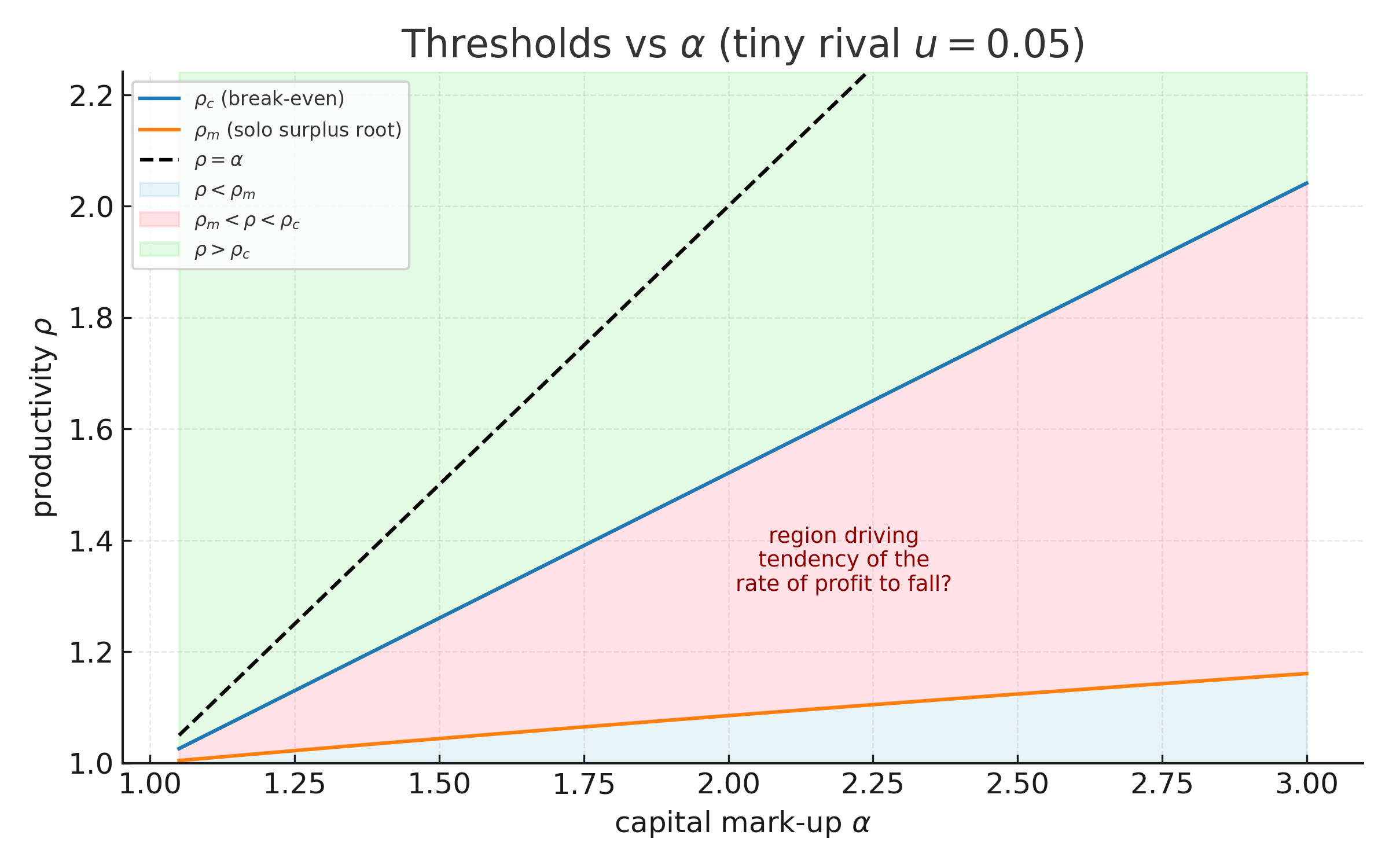
 ).
). .
.
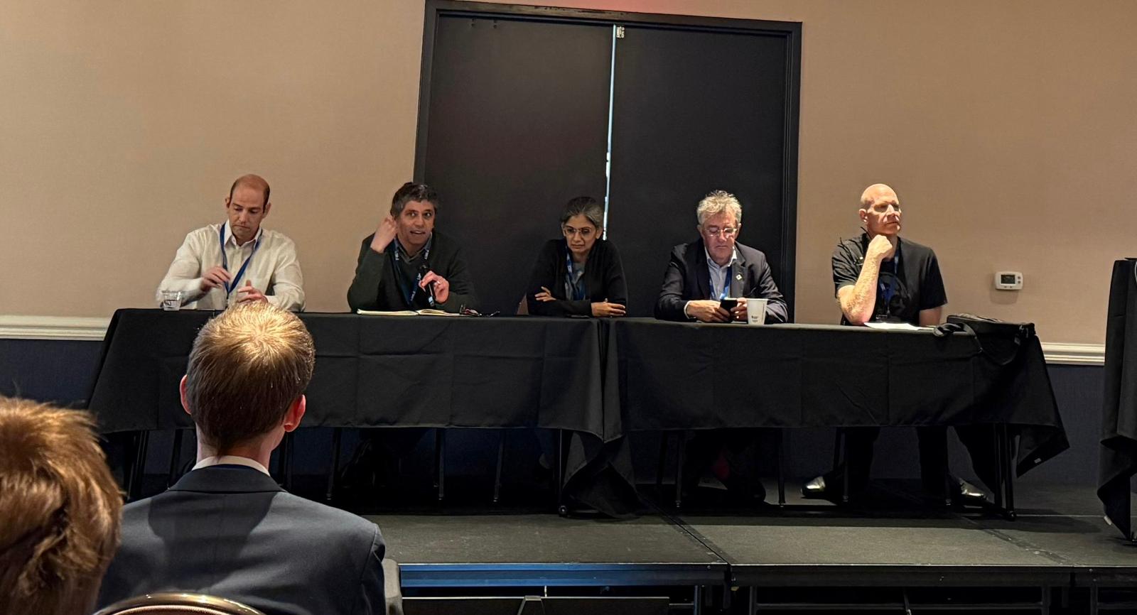
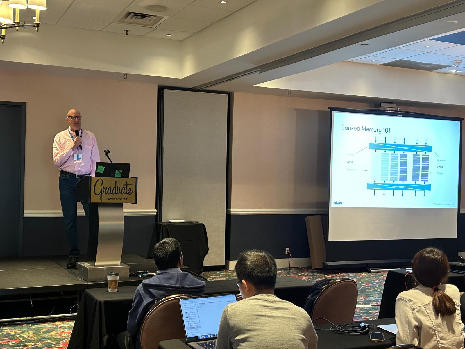
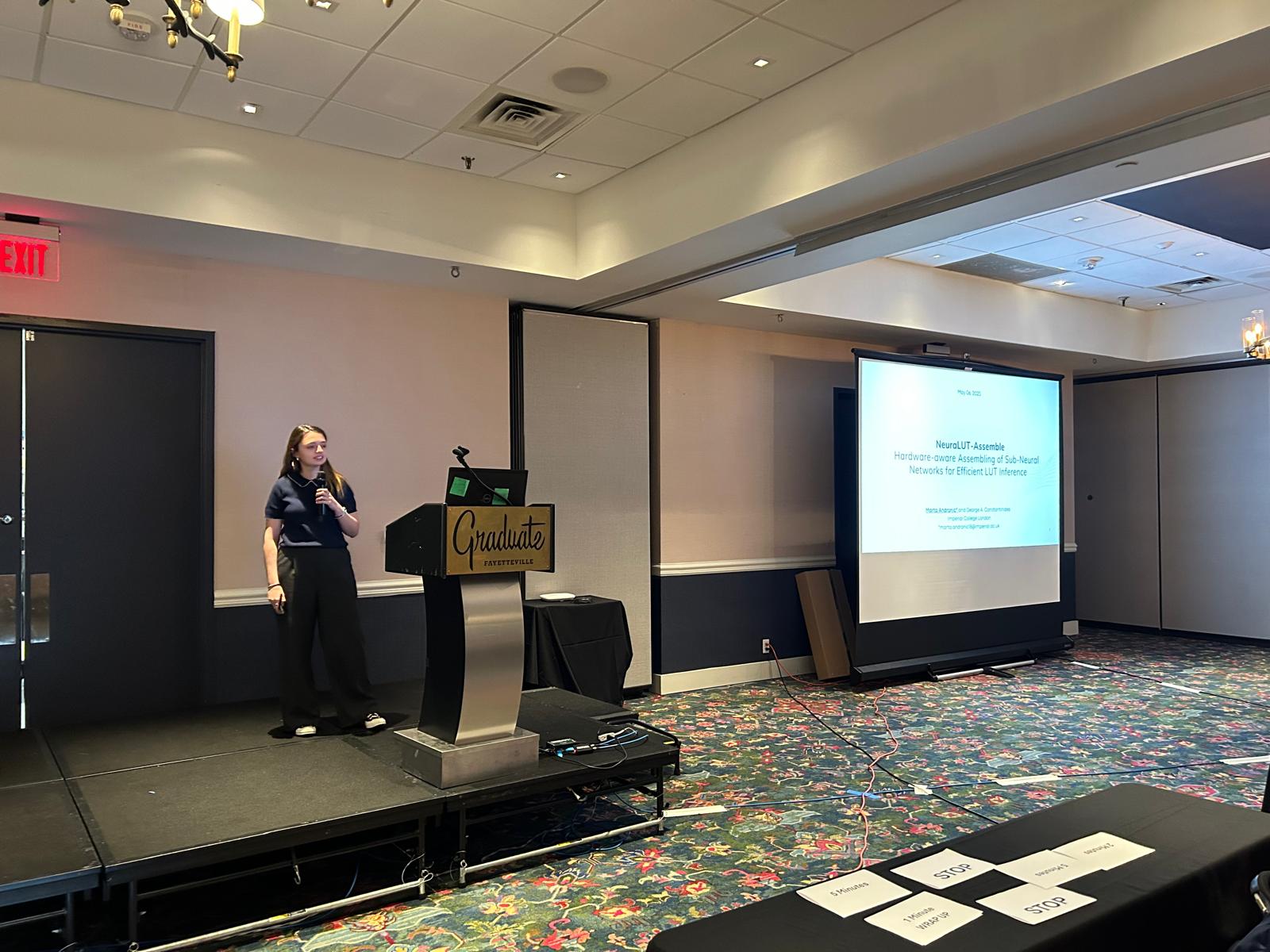
 -out-of-
 element sparsity in tensor processing tiles.
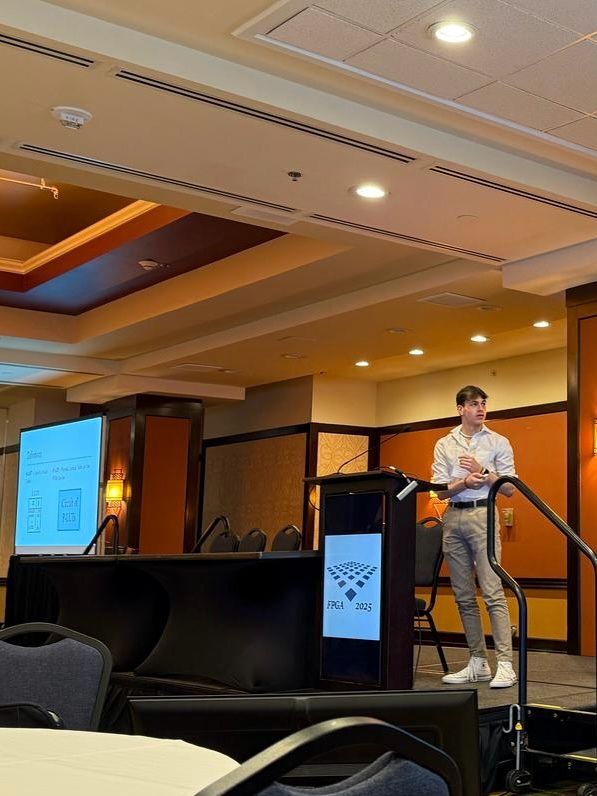
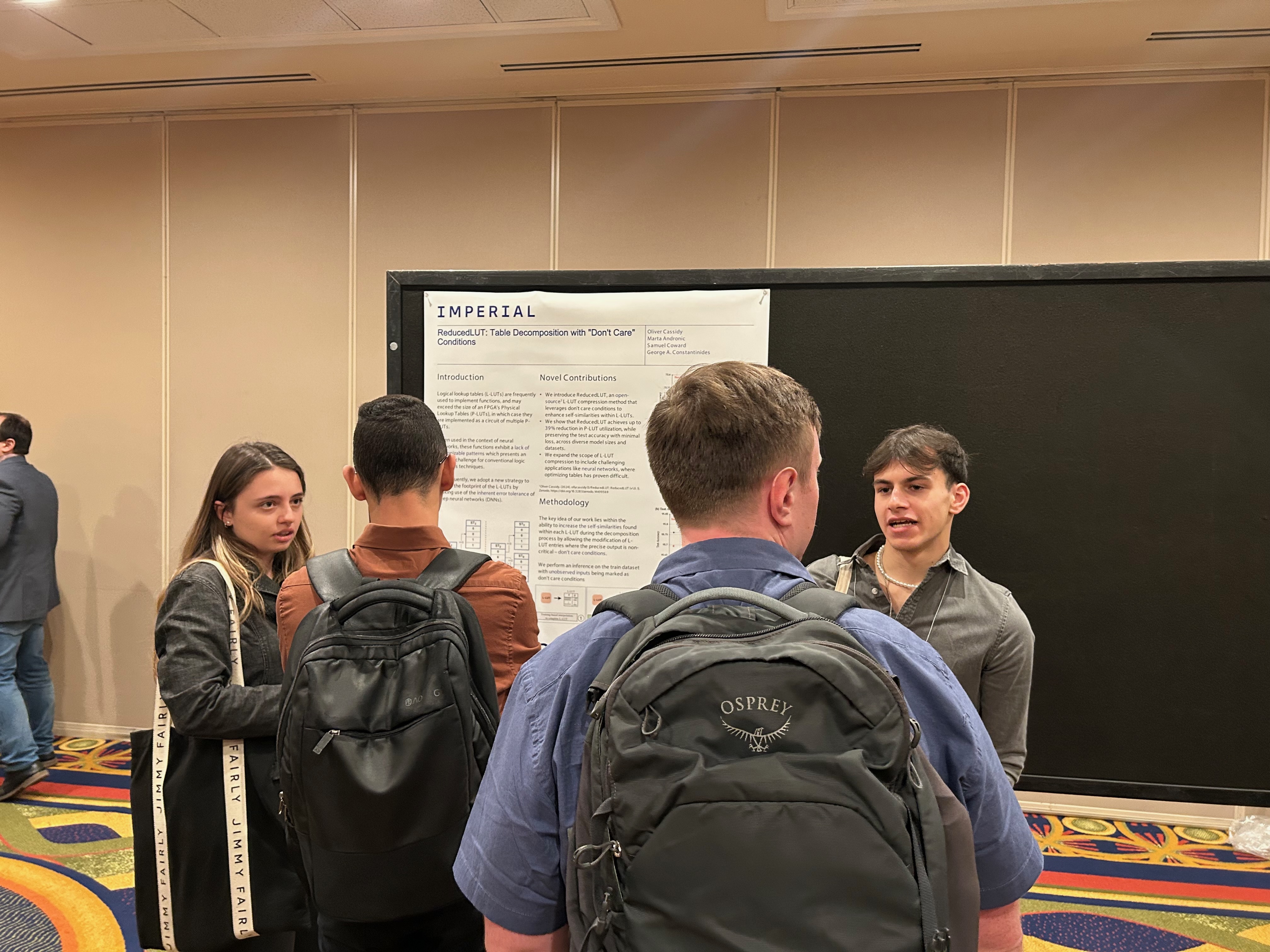
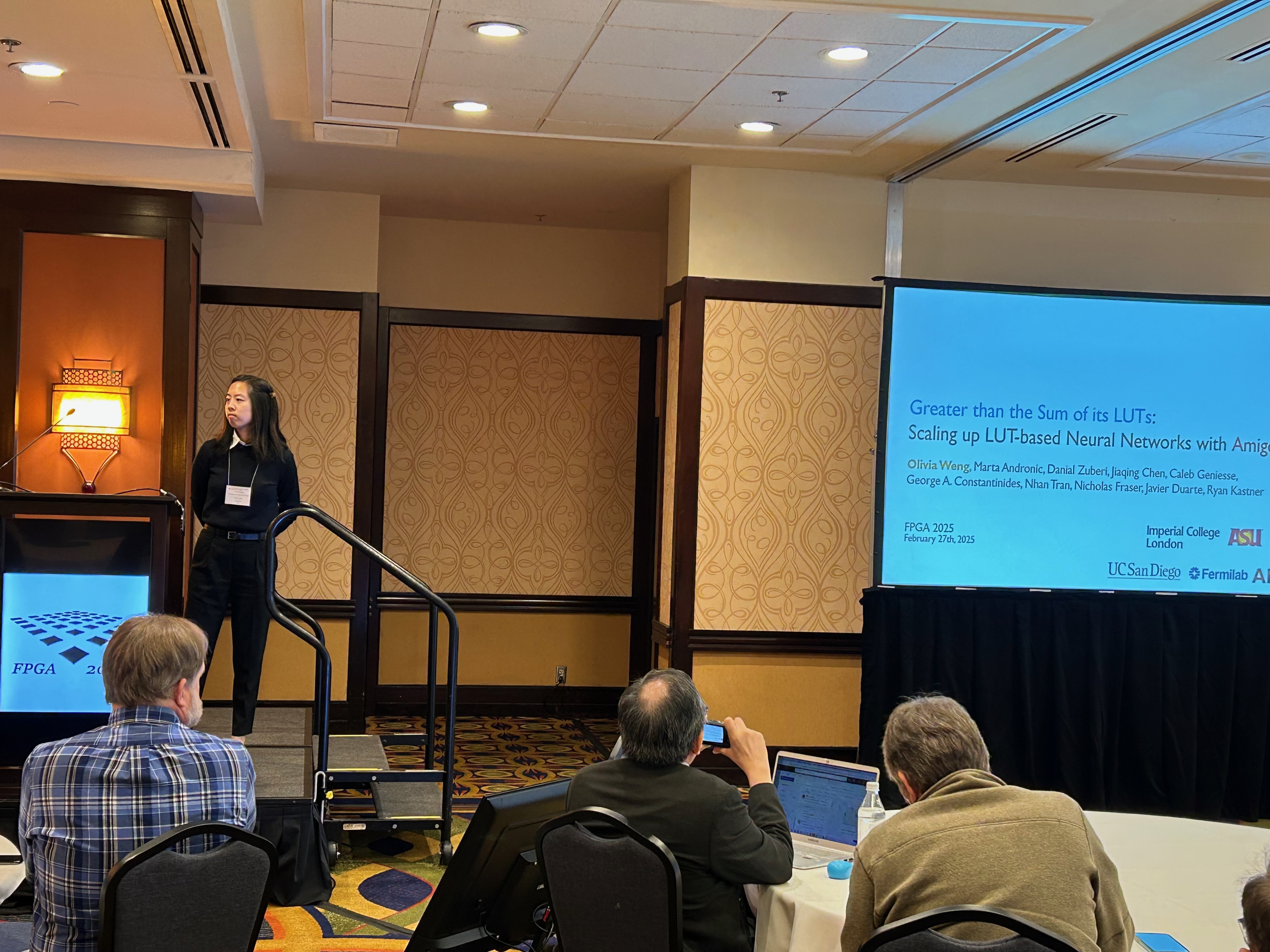
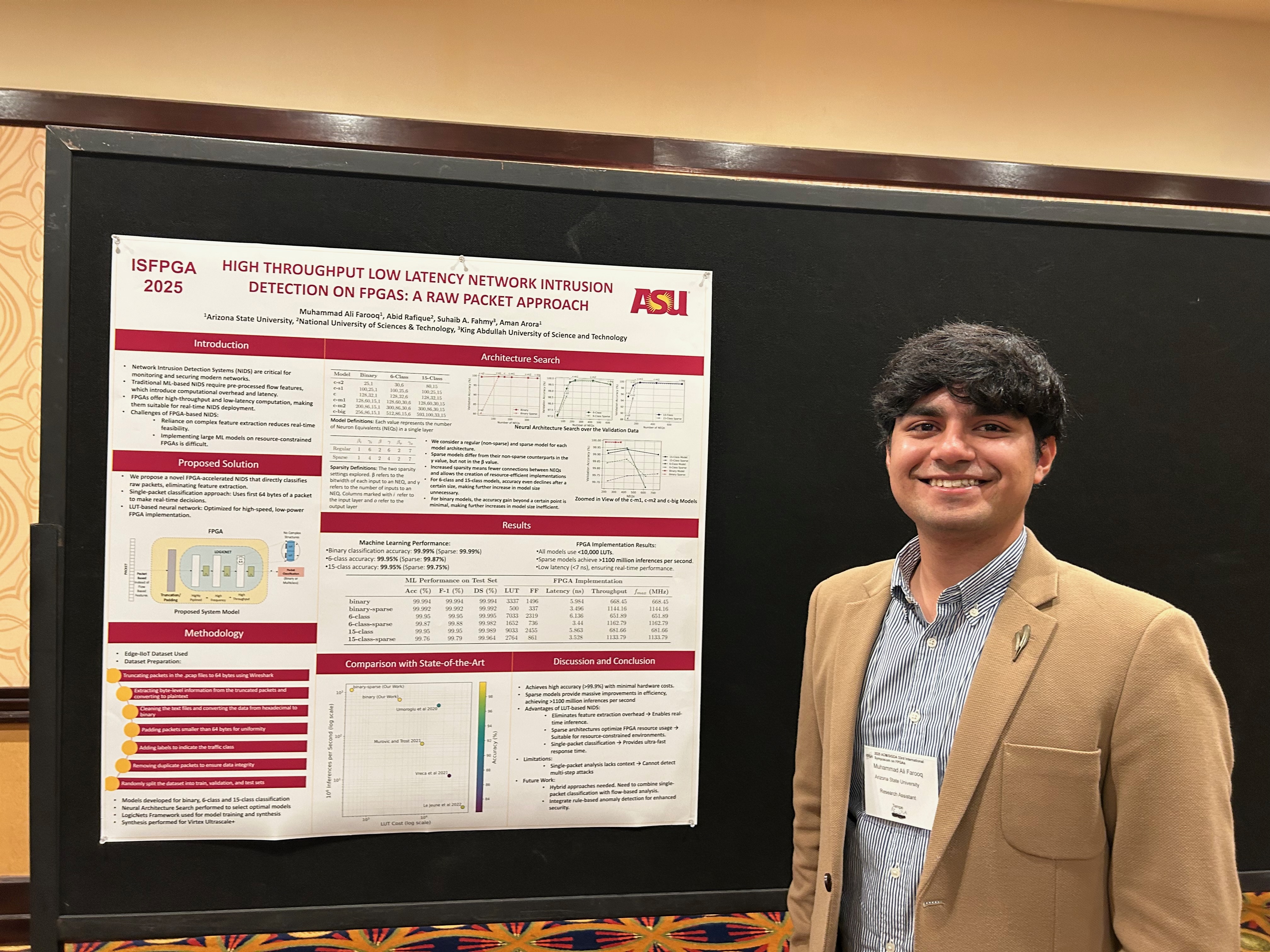
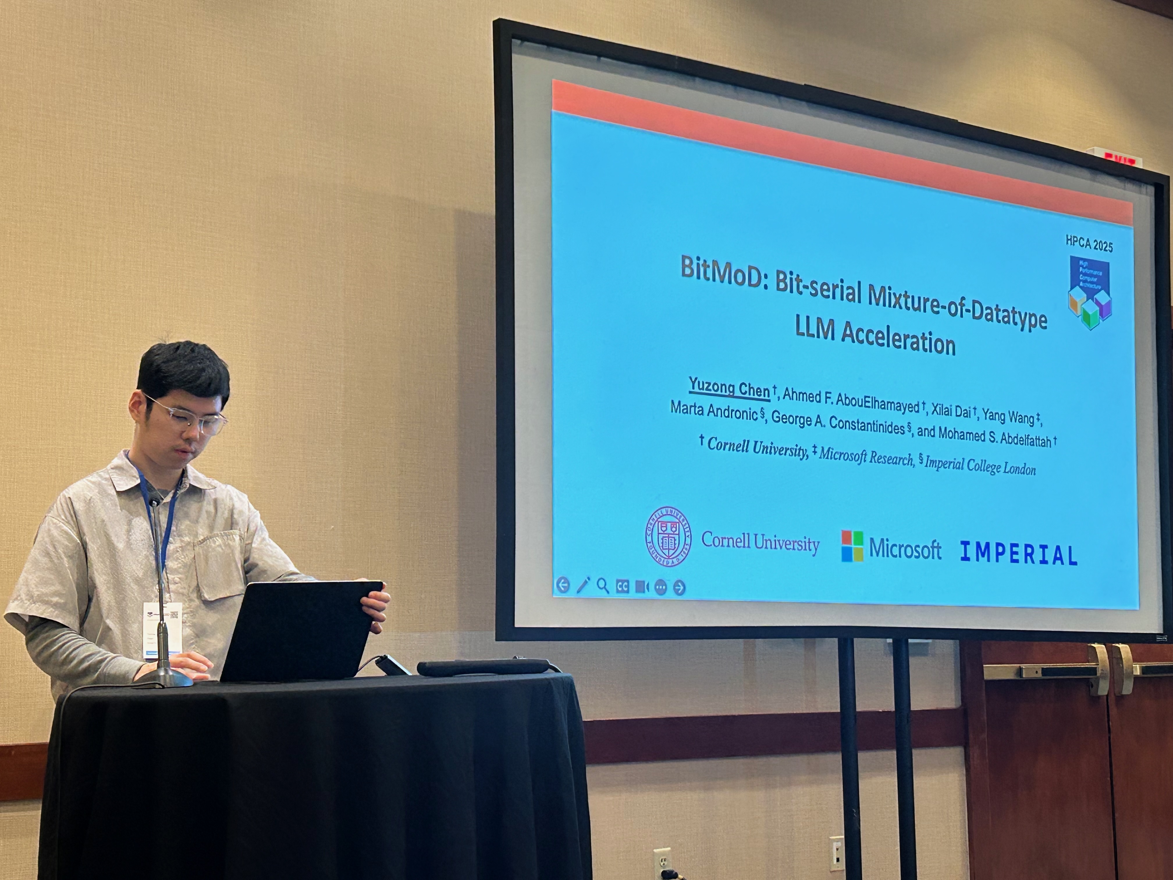
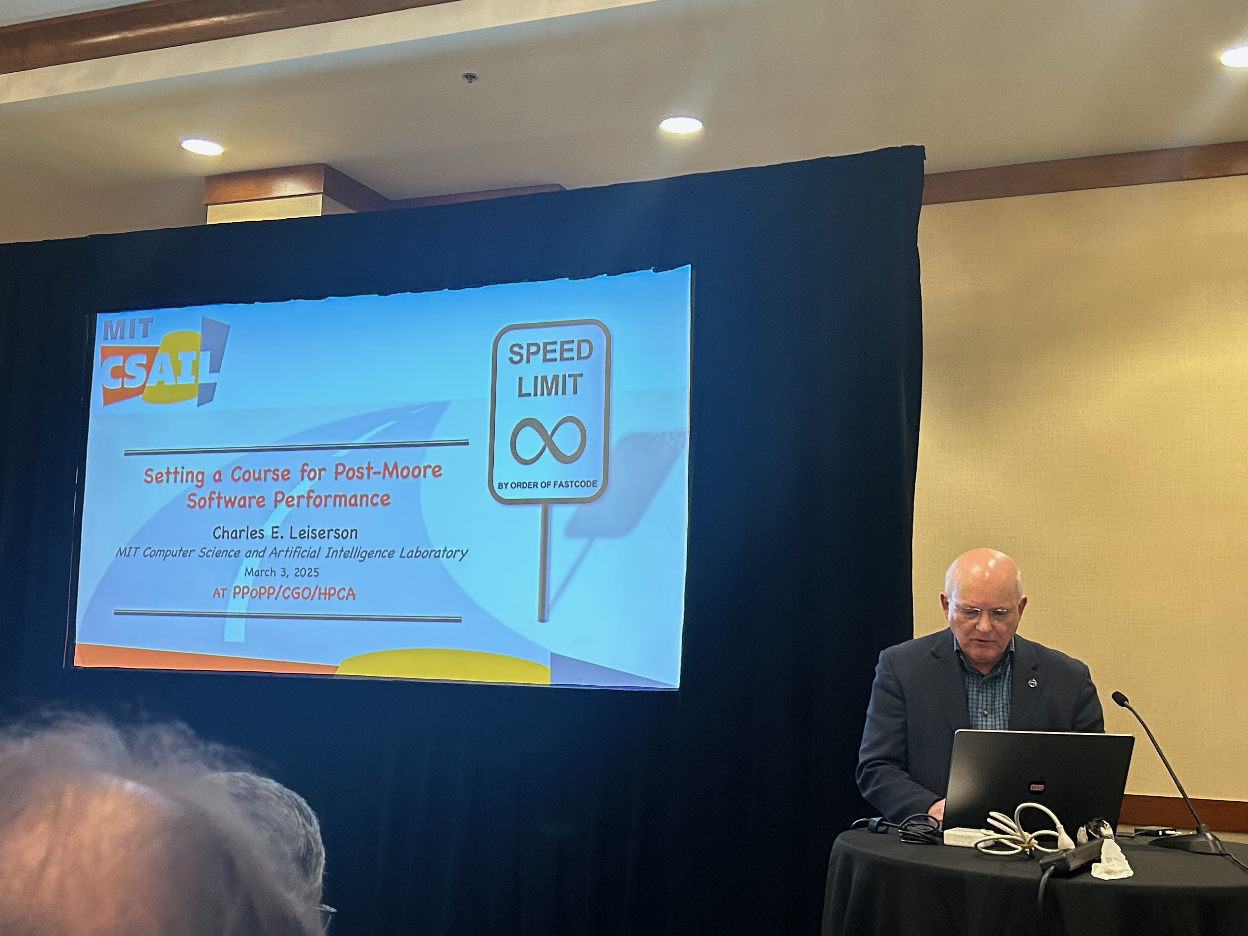

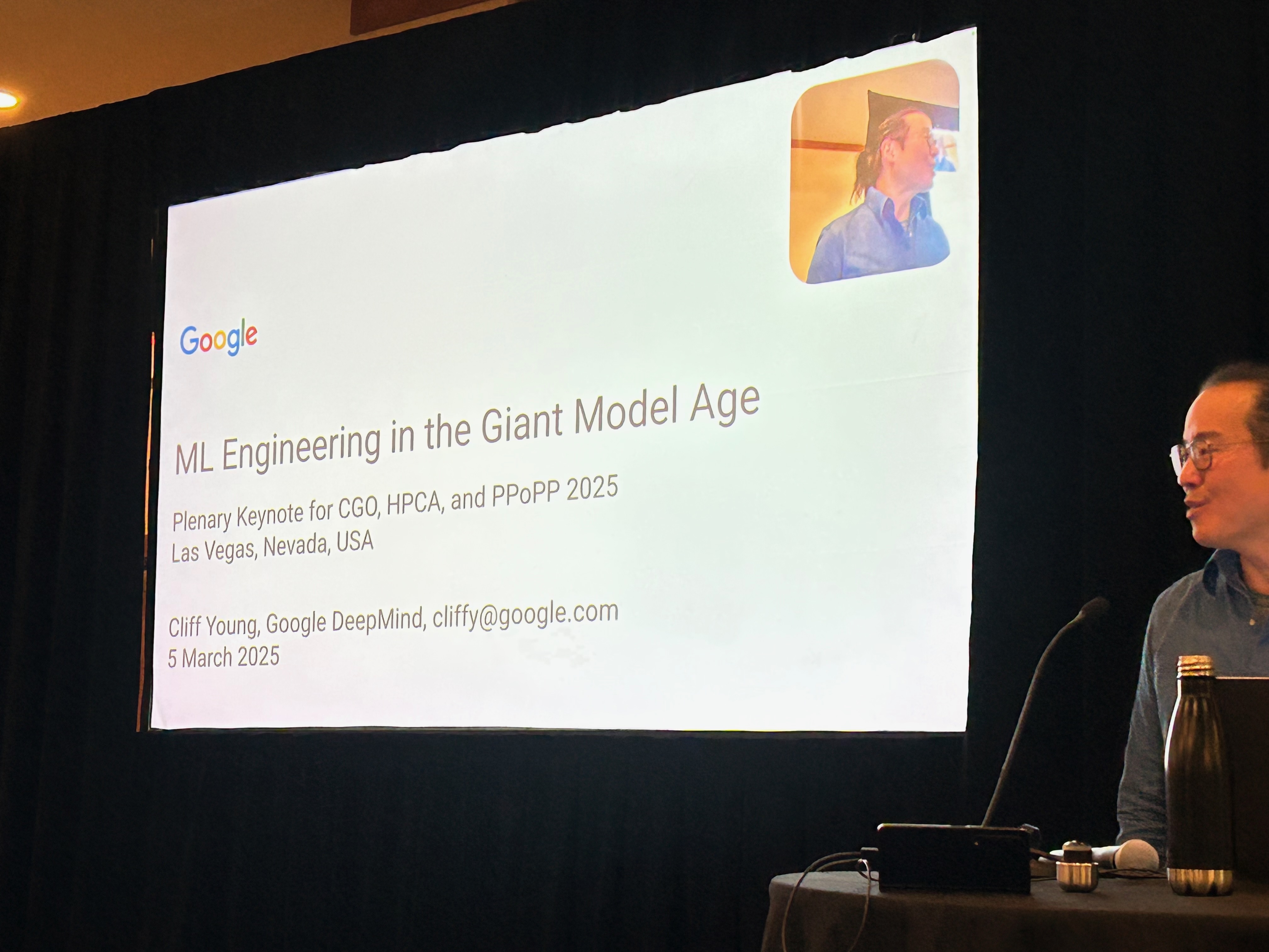
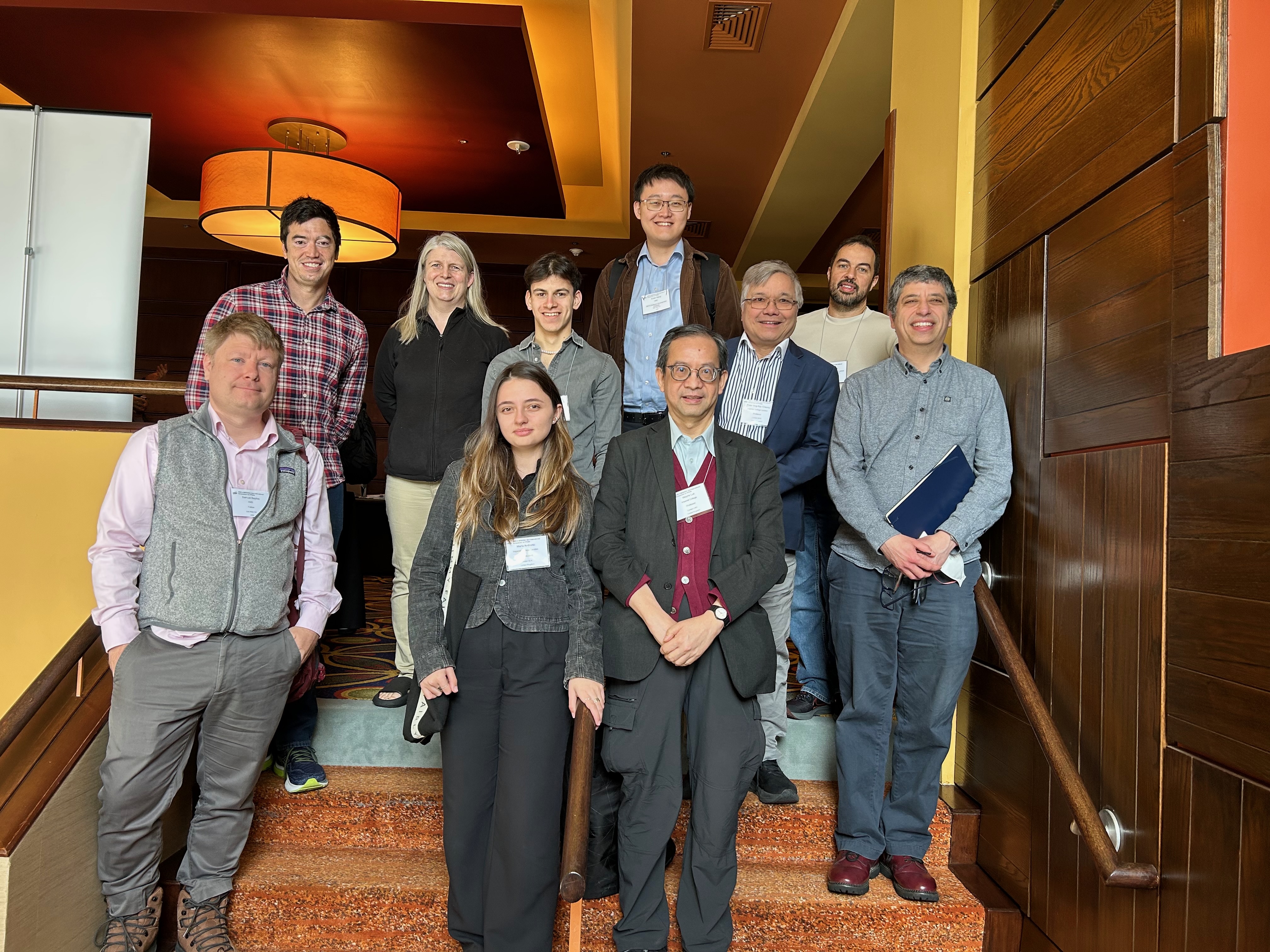

 -input Boolean function, then learn all
  lines in that function’s truth table. Since then, Marta and I have been exploring ways of parameterising that space to decouple the complexity of the function-classes implemented from the number of inputs. This gave rise to PolyLUT (parameterised as polynomials) and NeuraLUT (parameterised as small neural networks). Once we have learnt a function
  , all these methods enumerate the inputs of the function for the discrete space of quantised activations to produce the L-LUT. Olly’s work introduces `don’t cares’ into the picture: if a particular combination of inputs to the function is never, or rarely, seen in the training data, then the optimisation is allowed to treat the function as a don’t care at that point.