politics – Thinking

This blog post sets up and analyses a simple mathematical model of Marx’s controversial “Law of the Tendency of the Rate of Profit to Fall” (Capital III §13-15). We will work under a simple normalisation of value that directly corresponds to the assumption of a fixed labour pool combined with the labour theory of value (LTV). I will make no remarks on the validity of LTV in this post, but all results are predicated on this assumption. We will also work in the simplest possible world of two firms, each generating baskets containing both means of production and consumer goods, and in which labour productivity equally improves productivity in the production of both types of goods. I will provide the mathematical derivations in sufficient detail that a sceptical reader can reproduce them quite easily with pen and paper.

The key interesting results I am able to derive here are:

If constant capital grows without bound, then the rate of profit falls, independently of any assumption on the rate of surplus value (a.k.a. the rate of exploitation).
There is a critical value of productivity $\rho_c$ (which we derive), above which innovation across firms raises the rate of profit of both firms, and below which the rate of profit is reduced.
There are investments that could be made by a single firm to raise its own productivity high enough to improve its own rate of profit when the competing firm does not change its production process. (We locate this threshold, $\rho_*$ ). However, none of these investments would reduce the rate of profit of when rolled out across both firms (i.e. $\rho_c < \rho_*$ ). There is therefore no “prisoner’s dilemma” of rates of profit causing capital investment to ratchet up.
However, a firm motivated by increasing its mass of profit (equivalently, its share of overall surplus value) is motivated to invest in productivity above a third threshold $\rho_m$ , which we also prove exists, and show that $\rho_m < \rho_c$ . Thus there is a range of investments that improve the profit mass of a single firm but also reduce the rate of profit when rolled out to both firms.

As a result, under the assumptions with which I am working, we can interpret Marx’s Law of the Tendency of the Rate of Profit to Fall to be an accurate summary of economic evolution in purely value terms, under the assumption that firms often seek out moderately productivity-enhancing innovations, so long as radically productivity-enhancing innovations are rare.

1. The Law of the Tendency of the Rate of Profit to Fall

Marx famously argued that the very innovations that make labour more productive eventually pull the average rate of profit downward. My understanding as a non-economist is that, even in Marxian economic circles, this law is controversial. Over my summer holiday, I have been reading a little about this (the literature is vast) and there are many complex arguments on both sides, often very wordy or apparently relying on assumptions that do not line up with a simple LTV analysis.

The aim of this post is thus to show, in the simplest possible algebra, how perfectly reasonable investment decisions by competitive firms reproduce Marx’s claim, providing explicit analysis for how the scale of productivity gains impact on the rate of profit and on individual motivating factors for the firms involved.

2. Set-up and notation

I will be working purely in terms of value, as I understand it from Capital Volume 1, i.e. socially necessary labour time (SNLT) – I will pass a very brief comment on price at the end of the post. We will use the following variables throughout the analysis, each with units of “socially necessary labour time per unit production period”.

Symbol	Definition	Economic reading in Capital
$C \geq 0$	overall constant capital	machinery + materials
$V \geq 0$	overall variable capital	value of wages
$S$	overall surplus value	unpaid labour
$c_i$	constant capital advanced by Firm i	machinery + materials
$v_i$	variable capital advanced by Firm i	value of wages

In addition, we will consider the following dimensionless scalar variables:

Symbol	Definition	Economic reading in Capital
$u > 0$	The baseline production rate of commodities by Firm 2, as a multiple of that produced by Firm 1
$\alpha > 1$	capital deepening factor: the ratio of the post-investment capital advanced to the pre-investment capital advanced, evaluated in terms of SNLT at the time of investment	dearer machine (III §13)
$\rho > 1$	labour-productivity factor: the ratio of the number of production units produced per unit production time post-investment to the same quantity prior to the investment.	fewer hours per unit (III §13)

We will work throughout under the constraint that $V + S = 1$ . This can be interpreted as Marx’s “limits of the working day” (Capital I §7) and flows directly from the LTV. Below I will refer to this as “the working day constraint”.

Before embarking on an analysis of productivity raising, it is worth understanding the rate of profit at an aggregate level. Marx defined the rate of profit as:

$r = \frac{S}{C+V}$

During my reading on the rate of profit, I have seen a number of authors describe the tendency of the rate to fall in the following terms: divide numerator and denominator by $V$ , to obtain $r = \frac{\frac{S}{V}}{1 + \frac{C}{V}}$ . At that point an argument is sometimes made that keeping $\frac{S}{V}$ (the rate of surplus labour, or the rate of exploitation) constant (or bounded from above), $r \to 0$ as as $\frac{C}{V} \to \infty$ . This immediately raises two questions: why should $\frac{S}{V}$ remain constant (or bounded), and why should $\frac{C}{V} \to \infty$ ? In this post, I will attempt to show that the first of these assumptions is irrelevant, while providing a reasonable basis to understand the second. As a prelude, we will now prove the following elementary theorem:

Theorem 1 (Rate of Profit Declines with Increasing Capital Value). Under the working-time constraint, $C \to \infty \Rightarrow r \to 0$ .

Proof. $r = \frac{S}{C+V} \leq \frac{1}{C} \to 0$ . □

It is worth noting that $C \to \infty$ implies that $\frac{C}{V} \to \infty$ , but the latter is not sufficient for $r \to 0$ – a simple counterexample would be to keep $C$ constant while $V \to 0$ , leading to an asymptotic rate of profit of $\frac{1}{C}$ .

Theorem 1 forms our motivation to consider why we may see $C$ increasing without bound. To understand this, we will be considering three scenarios:

Scenario A: the baseline. Each firm is producing in the same way, but they may have a different scale of production. We will normalise production of Firm 1 to 1 unit of production, with Firm 2 producing $u$ units of production per unit production time.

Scenario B: after a general rise in productivity. Each firm is again producing in the same way, with the same ratio of production units as Scenario A. Each firm has, however, made the same productivity-enhancing capital investment, so that Firm 1 is now producing $\rho$ units and Firm 2 is now producing $\rho u$ units of production per unit time.

Scenario C: only a single firm, Firm 1, implements the productivity-enhancing capital investment. Firm 1 is now producing $\rho$ units and Firm 2 is still producing $u$ units of production per unit time. This scenario allows us to explore differences in rate and mass of profit for Firm 1 compared to Scenario A and Scenario B, proving several of the results mentioned at the outset of this post.

3. Scenario A — baseline

We have: $V = (1+u)v_1$ and $C = (1+u)c_1$ .

The total value of the units of production produced is $C + V + S = C + 1 = 1 + (1+u)c_1$ (using the working day constraint). Each unit of production therefore has a value of $\frac{1}{1+u} + c_1$ . Firm 1 is producing 1 of these units.

The surplus value captured by (profit mass of) Firm 1 is therefore $s_1 = \frac{1}{1+u} - v_1$ .

This gives an overall rate of profit for Firm 1 of: $r_1 = \frac{s_1}{c_1 + v_1} = \frac{1 - (1+u)v_1}{(1+u)(c_1+v_1)}$ .

This rate of profit is the same for Firm 2, and indeed for the overall combination of the two. We now have a baseline rate and mass of profit, against which we will make several comparisons in the next two scenarios.

4 Scenario B — both firms upgrade

In this scenario, both firms upgrade their means of production, leading to productivity boost by a factor of $\rho$ , after an increase in the value of capital advanced by a factor of $\alpha$ . We will assume that the firms keep the number of working hours constant, and ‘recycle’ the productivity enhancement to produce more goods rather than to drop the labour time employed.

We must carefully consider the impact on the value of variable and fixed capital of this enhancement. The value of variable capital has decreased by a factor $\rho$ , because it is now possible to meet the same consumption needs of the workforce with this reduced SNLT. Of course, we could make other assumptions, e.g. the ability of the labour force to ‘track’ productivity gains in terms of take-home pay, but the assumption of fixed real wages appears to be the most conservative reasonable assumption when it comes to demonstrating the fall of the rate of profit. Equally, the value of the fixed capital has reduced from the original $c_i$ for Firm $i$ to $\frac{\alpha c_i}{\rho}$ , because a greater investment has been made at old SNLT levels ( $\alpha > 1$ ) but this investment has itself depreciated in value due to productivity gains. Marx refers to this as ‘cheapening’ in Capital III §14.

We will use singly-primed variables to denote the quantities in Scenario B, in order to distinguish them from Scenario A. We have:

$C' = \frac{\alpha (1+u)}{\rho}c_1$

The total value of the units of production produced is $C' + V' + S' = 1 + C' = 1 + \frac{\alpha (1+u)}{\rho}c_1$ . Remembering that our firms together now produce $\rho(1+u)$ units of production, each unit therefore has value $\frac{1}{\rho(1+u)} + \frac{\alpha}{\rho^2}c_1$ .

Firm 1 is responsible for $\rho$ of these units, and therefore a value of $\frac{1}{1+u} + \frac{\alpha}{\rho}c_1$ . We may therefore calculate the portion of surplus labour it captures as:

$s'_1 = \frac{1}{1+u} - \frac{1}{\rho}v_1$ , and its rate of profit as:

$r'_1 = \frac{\frac{1}{1+u} - \frac{v_1}{\rho}}{\frac{\alpha}{\rho}c_1 + \frac{1}{\rho}v_1}$ .

Simplifying, we have

$r'_1 = \frac{\rho - (1+u)v_1}{(1+u)(\alpha c_1 + v_1)}$ .

These will be the same rate for Firm 2 (and overall) and a proportionately scaled mass for Firm 2.

It is clear that $s'_1 > s_1$ , i.e. profit mass is always increased by universally adopting an increased productivity (remember we are keeping real wages constant). However, it is not immediately clear what happens to profit rate.

Theorem 2 (Critical productivity rate for universal adoption). For any given set of variables from Scenario A, there exists a critical productivity rate $\rho_c = 1 + (\alpha - 1)(1 - V)\frac{c_1}{c_1+v_1} < \alpha$ . We have $r'_1 > r_1$ iff $\rho > \rho_c$ .

Proof. Firstly, we will establish that $\rho_c < \alpha$ . This follows from the fact that $1-V$ and $\frac{c_1}{c_1+v_1}$ are both strictly less than 1.

Now $r'_1 > r_1$ iff $\dfrac{\rho-(1+u)v_1}{(1+u)(\alpha c_1+v_1)} \;>\; \dfrac{1-(1+u)v_1}{(1+u)(c_1+v_1)}$ . Clearing (positive) denominators and noting $V = (1+u)v_1$ gives the equivalent inequality $\rho(c_1 + v_1) - (\alpha c_1 + v_1) - (1 - \alpha)Vc_1 > 0$ . Isolating $\rho$ gives $\rho > \frac{\alpha c_1 + v_1 - (\alpha - 1)Vc_1}{c_1 + v_1} = \rho_c$ . □

The the overall rate of profit in Scenario 2 can rise or fall, depending on the level of productivity those gains bring. The more the cost of the new means of production, the less is spent on wages, and the greater the fixed-capital intensive nature of the production process, the higher the productivity gain required to reach a rise in profit rate, arguably raising the critical threshold as capitalism develops. However, the fact that and that $\rho_c < \alpha$ indicates it will always raise the rate of profit to invest in a productivity gain that’s more than the markup in capital required to implement that gain. That it is still beneficial for the overall rate of profit to adopt productivity gains less significant than the markup in capital expenditure, i.e. when $\rho_c < \rho < \alpha$ , appears to be consistent with Marx’s Capital III §14, where he appears to be assuming this scenario.

5 Scenario C — Firm 1 upgrades alone

We are interested in now exploring a third scenario: the case where Firm 1 implements a way to increase its own productivity through fixed capital investment, but this approach is kept private to Firm 1. This scenario is useful for understanding cases that may motivate Firm 1 to improve productivity and to understand to what degree they differ from the cases motivating both firms to improve productivity by the same approach.

As per Scenario B, it is important to understand the changes to the SNLT required in production. In Capital I §1, it is clear that Marx saw this as an average. A suitable cheapening factor for labour in these circumstances is $\frac{u+1}{\rho+u}$ because with the same labour ( $V+S=1$ ) as in Scenario A, we have gone from the overall social production of $u+1$ units of production ( $u$ from Firm 2 and 1 from Firm 1), to $u+\rho$ units of production.

In this scenario we will use doubly primed variable names to distinguish the variables from the former two scenarios. We will begin, as before, with fixed capital, noting that both firms’ capital and labour has cheapened through the change in SNLT brought about by the investment of Firm 1, however Firm 1 also bears the cost of that investment:

$c_1'' = \alpha c_1 \frac{u+1}{\rho+u}$ and $c_2'' = u c_1 \frac{u+1}{\rho+u}$ .

$C'' = c_1'' + c_2'' = c_1(\alpha+u)\frac{u+1}{\rho+u}$ .

The total value of the units of production produced by both firms during unit production time is now $V'' + S'' + C'' = 1 + C'' = 1 + c_1(\alpha+u)\frac{u+1}{\rho+u}$ .

This means that since $\rho+u$ units of production are being produced, each unit of production now has value $\frac{1}{\rho + u} + c_1\frac{(u+1)(\alpha+u)}{(\rho+u)^2}$ . As we did for Scenario B, we can now compute the value of the output of production of Firm 1 by scaling this quantity by $\rho$ , obtaining output value $\frac{\rho}{\rho + u} + c_1 \frac{\rho(u+1)(\alpha+u)}{(\rho+u)^2}$ . We may then calculate the surplus value captured by Firm 1 by subtracting the corresponding fixed and variable capital quantities, remembering that both have been cheapened by the reduction in SNLT:

$s_1'' = \frac{\rho}{\rho + u} + c_1 \frac{\rho(u+1)(\alpha+u)}{(\rho+u)^2} - c_1 \frac{\alpha(u+1)}{\rho+u} - \frac{(u+1)v_1}{\rho+u}$

$= \frac{\rho - (u+1)v_1}{\rho+u} + c_1 \frac{u(u+1)(\rho - \alpha)}{(\rho+u)^2}$ .

The first term in this profit mass expression simply reveals the revalued living labour contributed. The second term is intriguing. Why is there a term that depends on fixed capital value when considering the profit mass under the labour theory of value? Under the assumptions we have made, this happens because although fixed-capital-value-in = fixed-capital-value-out at the economy level, this is no longer true at the firm level; this corresponds to a repartition of SNLT in the market between Firm 1 and Firm 2, arising due to the fundamental assumption that each basket of production has the same value, independently of how it has been made. It is interesting to note that this second term, corresponding to revalued capital, changes sign depending on the relative magnitude of $\rho$ and $\alpha$ . For $\rho > \alpha$ , the productivity gain is high enough that Firm 1 is able to (also) boost its profit mass by capturing more SNLT embodied in the fixed capital, otherwise the expenditure will be a drag on profit mass, as is to be expected.

Now we have an explicit expression for $s_1''$ , we may identify the circumstances under which profit mass rises when moving from Scenario A to Scenario C.

Theorem 3 (Critical Productivity Rate for Solo-Profit Mass Increase). For any given set of variables from Scenario A, there exists a critical productivity rate $\rho_m < \alpha$ for which we have $s''_1 > s_1$ iff $\rho > \rho_m$ .

Proof. We will begin by considering the difference between surplus value captured in Scenario C and that captured in the baseline Scenario A. We will consider this as a function $\Theta$ of $\rho$ .

$\Theta(\rho) := s_1'' - s_1 = \frac{\rho - (u+1)v_1}{\rho + u} + c_1 \frac{u(u+1)(\rho-\alpha)}{(\rho+u)^2} - \left( \frac{1}{u+1} - v_1 \right)$ .

Differentiating with respect to $\rho$ ,

$\frac{d\Theta}{d\rho} = \frac{u+(u+1)v_1}{(\rho + u)^2} + c_1 u (u+1) \frac{2\alpha + u -\rho}{(\rho+u)^3}$ .

Both denominators are positive. The first numerator is clearly positive. The second numerator is also positive for $\rho \in (1,\alpha)$ . Hence $\Theta$ is strictly increasing over the interval $(1,\alpha)$ .

Now note that as $\rho \to 1^+$ , $\Theta(\rho) \to c_1 u \frac{1-\alpha}{u+1} < 0$ . However, at $\rho = \alpha$ , $\Theta(\alpha)$ simplifies to $\Theta(\alpha) = \frac{(\alpha - 1)\left[ u+ (1+u)v_1 \right]}{(\alpha + u)(u + 1)} > 0$ . Hence by the intermediate value theorem and strict monotonicity there is a unique value $\rho_m$ with $1 < \rho_m < \alpha$ such that $\rho > \rho_m$ iff $s_1'' > s_1$ . □

At this point, it is worth understanding where this critical profit-mass inducing productivity increase lies, compared to the value $\rho_c$ we computed earlier as the minimum required productivity increase in Scenario B required to improve the rate of profit. It turns out that this depends on the various parameters of the problem. However, a limiting argument shows that for large Firm 1, any productivity enhancement will improve profit mass, whereas for small Firm 1 under sufficiently fixed-capital-intensive production, only productivity enhancements outstripping capital deepening would be sufficient:

Theorem 4 (Limiting Firm Size and Solo-Profit Mass). As $u \to 0^+$ , $\Theta(\rho) \to v_1 \left( 1 - \frac{1}{\rho} \right)$ . As $u \to \infty$ , $\Theta(\rho) \to \frac{1}{u}\left( \rho - 1\right) + c_1(\rho - \alpha)$ .

Proof. Both statements follow by direct substitution into the expression for $\Theta$ given in the proof of Theorem 3 and taking limits. □

It is worth dwelling briefly on why there is this dichotomous behaviour between large and small firms. A large Firm 1 ( $u \to 0$ ) has an output that dominates the value of the product; it takes the lion share of SNLT, and the only impact on the firm of raising its productivity is to reduce the value of labour power as measured in SNLT, which will always be good for the firm. However, a small Firm 1 ( $u \to \infty$ ) has no impact on the value of the product or of labour power. It is certainly able to recover more overall value from the products in the market (the term $\frac{1}{u}\left( \rho - 1\right) > 0$ ), but it must carefully consider its outlay on fixed-capital. In particular if $\rho < \alpha$ , only small $c_1$ – a low capital intensity – would lead to a rise in profit mass.

So at least for large firms (or low capital intensity) there is a range of productivity enhancements $\rho_m < \rho < \rho_c$ that will induce a rise in profit mass for solo adopters (Scenario C) but would lead to a fall in the overall rate of profit when universally adopted (Scenario B).

It is now appropriate to consider the individual rate of profit of Firm 1 in Scenario C, having so far concentrated only on the mass of profit.

The rate of profit of Firm 1 in Scenario C is:

$r1'' = \frac{\frac{\rho - (1+u)v_1}{\rho+u} + c_1\frac{u(u+1)(\rho-\alpha)}{(\rho+u)^2}}{\frac{u+1}{\rho+u}(\alpha c_1 + v_1)} = \frac{\rho - (1+u)v_1+\frac{u(u+1)c_1(\rho-\alpha)}{\rho+u}}{(u+1)(\alpha c_1 + v_1)}$ .

As with the mass of profit, we are able to demonstrate the existence of a critical value of productivity, above which Firm 1 increases its rate of profit as a solo adopter:

Theorem 5 (Critical Productivity Rate for Solo-Profit Rate Increase). For any given set of variables from Scenario A, there exists a critical productivity rate $\rho_* < \alpha$ for which we have $r''_1 > r_1$ iff $\rho > \rho_*$ .

Proof. As per the proof of the profit mass case, we will firstly compute the difference between the two scenarios, which we will denote $\Phi(\rho) := r''_1 - r_1$ . Forming a common denominator $D := (u+1)(\alpha c + v_1)(c_1 + v_1)$ that does not depend on $\rho$ between the expressions for $r''_1$ and $r_1$ allows us to write $\Phi(\rho) = N(\rho)/D$ where $N(\rho) := (c_1+v_1)\left[ \rho - (1+u)v_1 + \frac{u(u+1)c_1(\rho-\alpha)}{\rho+u} \right] - (\alpha c_1 + v_1)\left[ 1 - (1+u)v_1 \right]$ . Note that $N(\rho)$ is differentiable for $\rho > 0$ , with:

$\frac{dN}{d\rho} = (c_1+v_1)\left[ 1 + u(u+1)c_1\frac{u+\alpha}{(\rho+u)^2} \right] > 0$

Hence $\Phi(\rho)$ is strictly increasing with $\rho$ .

Now let’s examine the sign of $N(\rho)$ as $\rho \to 1$ . Firstly, by direct substitution, $N(\rho) \to (c_1+v_1) \left[ S + c_1 u (1-\alpha) \right] - (\alpha c_1 + v_1)S$ , where we have also recognised that $S$ , total surplus value in Scenario A, is $S = 1 - (1+u)v_1$ . This expression simplifies to $(1-\alpha)c_1 \left[S+ (c_1+v_1)u \right]$ . Of the three multiplicative terms, the first is negative ( $\alpha > 1$ ) while the other two are positive. Hence $N(\rho)$ becomes negative as $\rho \to 1$ , and hence so does $\Phi(\rho)$ .

We should also examine the sign of $N(\rho)$ at $\rho = \alpha$ . This time, $N(\alpha) = (c_1+v_1)\left[ \alpha - (1 - S) \right] - (\alpha c_1 + v_1) S$ , which simplifies to $N(\alpha) = (\alpha - 1)v_1\left[ 1+ c_1(1 + u) \right]$ . Since both multiplicative terms are positive, $N(\alpha)$ and hence $\Phi(\alpha)$ is positive.

So again we can make use of the intermediate value theorem, combined with our proof that $\Phi(\rho)$ is strictly increasing to conclude that there exists a unique $\rho_*$ such that $\Phi(\rho) > 0$ iff $\rho > \rho_*$ , completing the proof. We have already shown that that $\rho_* < \alpha$ via the second half of the sign-change argument. □

It remains, now, to try to place $\rho_*$ in magnitude compared to the other critical value we discovered, $\rho_c$ :

Theorem 6 (Productivity required for solo rate improvement dominates that required for universal rate improvement). $\rho_c < \rho_*$ .

Proof. We can place our earlier expressions for $r_1'$ and $r_1''$ over a common denominator $D' = (u+1)(\alpha c_1 + v_1) > 0$ that does not depend on $\rho$ . Here $r_1' = \frac{N'(\rho)}{D'}$ and $r_1'' = \frac{N''(\rho)}{D'}$ where $N'(\rho) := \rho - (1+u)v_1$ and $N''(\rho) := \rho - (1+u)v_1 + \frac{u(u+1)c_1(\rho-\alpha)}{\rho+u}$ .

Note that $N''(\rho) = N'(\rho) + \frac{u(u+1)c_1(\rho-\alpha)}{\rho+u}$ . Evaluating at $\rho = \rho_c$ , we have $N''(\rho_c) = N'(\rho_c) + \frac{u(u+1)c_1(\rho_c-\alpha)}{\rho_c+u}$ . From Theorem 2, we know that $\rho_c < \alpha$ and so the second term is negative and so $N''(\rho_c) < N'(\rho_c)$ .

Since $D$ was independent of $\rho$ and positive, we can conclude that $r_1''(\rho_c) < r_1'(\rho_c)$ . However, we also know that $r_1'(\rho_c) = r_1$ by definition of $\rho_c$ . Hence $r_1''(\rho_c) < r_1$ . And we may therefore conclude that $\rho_c < \rho_*$ . □

This theorem demonstrates that there is no “prisoner’s dilemma” when it comes to rate of profit in this model: if a firm is motivated to invest in order to raise its own rate of profit ( $\rho > \rho_*)$ then that investment will also raise overall rate of profit if implemented universally.

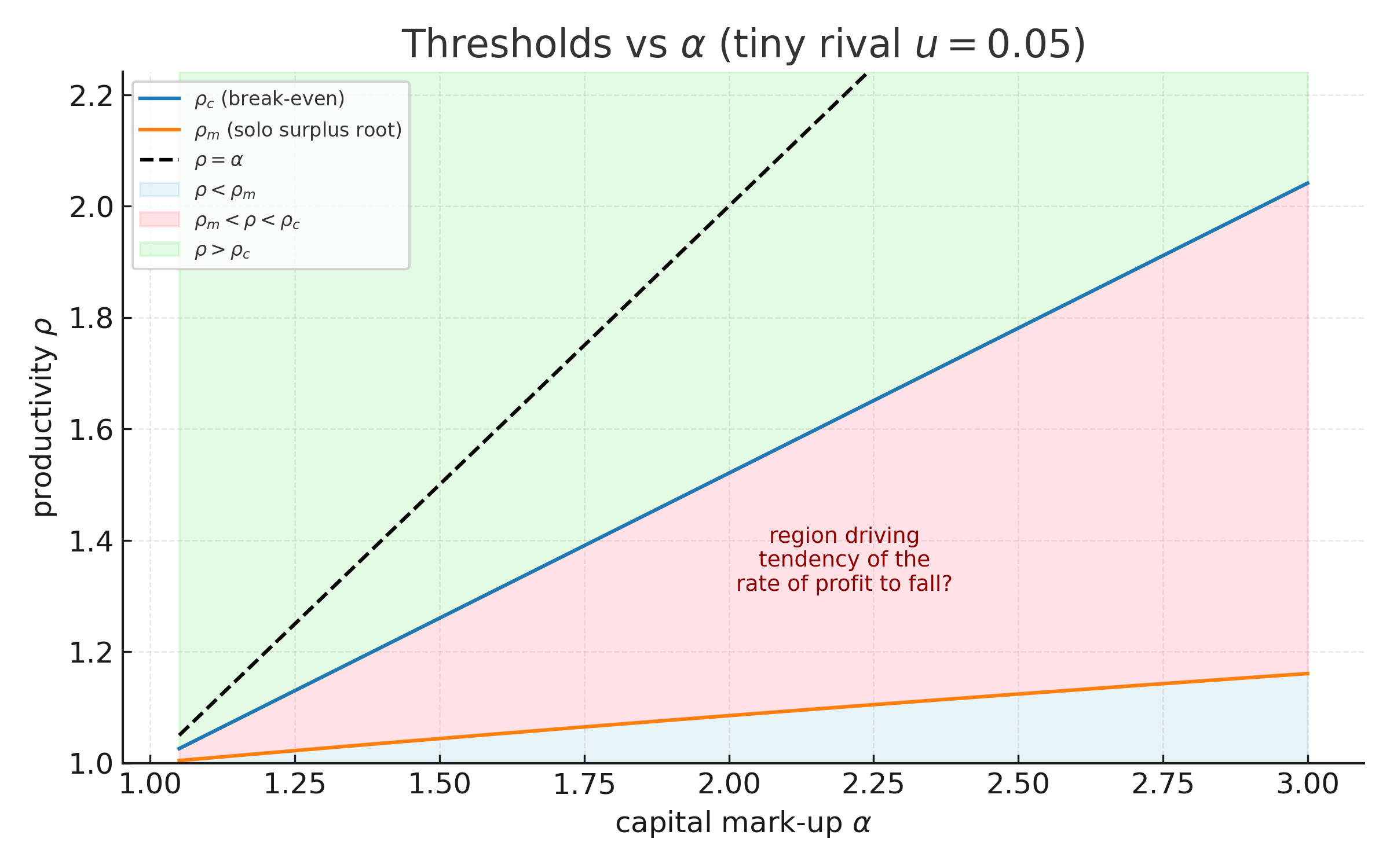
6. Summary of Thresholds

We have demonstrated a number of critical thresholds of productivity increase. Collecting results, we have

$\boxed{1 < \rho_c < \rho_* < \alpha}$

In the case of large firms (or production that is sufficiently low in fixed-capital input), we may also write:

$\boxed{1 < \rho_m < \rho_c < \rho_* < \alpha}$

A numerical example of these thresholds is illustrated below, for the large firm case.

Several conclusions flow from this order:

There are no circumstances under which a firm, to improve its rate of profit, makes an investment that will not also improve the rate of profit if universally adopted ( $\rho_* > \rho_c$ ).
There are cases, especially for large firms, where investments that may be attractive from the perspective of improving profit mass nevertheless reduce profit rate ( $\rho_m < \rho_c$ ).
There are productivity-enhancing investments that may be unattractive from a purely driven (either mass or rate).

7. Conclusion: The Falling Rate of Profit

In this model, we can conclude that continuous investment in moderately productivity-enhancing means of production ( $\rho < \alpha$ ) will lead to a falling rate of profit. Overall capital value $C$ will grow, which (Theorem 1) will lead to a falling rate of profit independent of assumptions on the rate of exploitation (rate of surplus value) $S/V$ .

The results in this post suggest that, if value after investment is considered by the investing firm, a key driver for this capital investment may not be the individual search for rate-of-profit enhancement by individual firms but rather simply a drive to increase their profit mass, capturing a larger proportion of overall surplus value, a situation particularly relevant under constraints on the total working time available (e.g. constrained population), and a common situation for large firms.

Some further remarks:

It is important to note that unlike a typical Marxian analysis, none of these results rely on the dislocation of price and value. Of course, it is quite plausible that the incentive to invest is based not on value but rather on current prices, but we have been able to show that such dislocation is not necessary to explain a falling rate of profit.
We have also not considered temporal aspects. It is possible that investment could be motivated by values before investment, leading to ‘apparent’ rates and masses of profit, rather than values after investment. To keep this post at a manageable length, I have not commented on this possibility, but again the aim has been to show that the falling rate can be explained without recourse to this.
We have not discussed the economic advantage that Firm 1 in Scenario 3 may have, e.g. being able to use its additional surplus value for power over the market. This may be an additional motivator for Firm 1 to move despite lower rate of profit, further accelerating the decline in the rate of profit.
Finally, as noted earlier in the post, we have preserved real wages in value after productivity enhancements, rather than allowed real wages to track productivity or benefit even slightly from productivity enhancement. This is a purposely conservative assumption, made as it seems the most hostile to retaining the falling rate of profit, and yet we still obtain a falling rate. If we allow wages to scale with productivity, this will of course further reduce the rate of profit.

I would very much welcome comments from others on this analysis, in particular over whether you agree that my analysis is consistent with Marx’s LTV framework.

Acknowledgements

The initial motivation for this analysis came from discussions with TG, YL and LW. I improved my own productivity by developing the mathematics and plot in this blog post using a long sequence of interactive sessions with the o3 model from OpenAI over a last week or so.

Update 28/6/25: The proof of Theorem 3 contained an error spotted by YL. This has now been fixed.

Update 12-13/7/25: Added further clarification of redistribution of value in Scenario C following discussion with YL and LW. Corrected an earlier overly simple precondition for $\rho_m < \rho_c$ spotted by YL.

Tag: politics

Do Your Best: A Social Question?

Responsibility and Causality

Mens Rea in the Information Age

From Omniscient Optimisation to Procedural Reasonableness

The Value of Social Norms

Trying One’s Best: A Practical Recipe

Acknowledgements

Productivity and Rate of Profit

1. The Law of the Tendency of the Rate of Profit to Fall

2. Set-up and notation

3. Scenario A — baseline

4 Scenario B — both firms upgrade

5 Scenario C — Firm 1 upgrades alone

6. Summary of Thresholds

7. Conclusion: The Falling Rate of Profit

Acknowledgements